
4.2 Data Warehouse Modeling: Data Cube and OLAP
Data warehouses and OLAP tools are based on a multidimensional data model. This model views data in the form of a data cube. In this section, you will learn how data cubes model n-dimensional data (Section 4.2.1). In Section 4.2.2, various multidimensional models are shown: star schema, snowflake schema, and fact constellation. You will also learn about concept hierarchies (Section 4.2.3) and measures (Section 4.2.4) and how they can be used in basic OLAP operations to allow interactive mining at multiple levels of abstraction. Typical OLAP operations such as drill-down and roll-up are illustrated (Section 4.2.5). Finally, the starnet model for querying multidimensional databases is presented (Section 4.2.6).
4.2.1 Data Cube: A Multidimensional Data Model
“What is a data cube?” A data cube allows data to be modeled and viewed in multiple dimensions. It is defined by dimensions and facts.
In general terms, dimensions are the perspectives or entities with respect to which an organization wants to keep records. For example, AllElectronics may create a sales data warehouse in order to keep records of the store’s sales with respect to the dimensions time, item, branch, and location. These dimensions allow the store to keep track of things like monthly sales of items and the branches and locations at which the items were sold. Each dimension may have a table associated with it, called a dimension table, which further describes the dimension. For example, a dimension table for item may contain the attributes item_name, brand, and type. Dimension tables can be specified by users or experts, or automatically generated and adjusted based on data distributions.
A multidimensional data model is typically organized around a central theme, such as sales. This theme is represented by a fact table. Facts are numeric measures. Think of them as the quantities by which we want to analyze relationships between dimensions. Examples of facts for a sales data warehouse include dollars_sold (sales amount in dollars), units_sold (number of units sold), and amount_budgeted. The fact table contains the names of the facts, or measures, as well as keys to each of the related dimension tables. You will soon get a clearer picture of how this works when we look at multidimensional schemas.
Although we usually think of cubes as 3-D geometric structures, in data warehousing the data cube is n-dimensional. To gain a better understanding of data cubes and the multidimensional data model, let’s start by looking at a simple 2-D data cube that is, in fact, a table or spreadsheet for sales data from AllElectronics. In particular, we will look at the AllElectronics sales data for items sold per quarter in the city of Vancouver. These data are shown in Table 4.2. In this 2-D representation, the sales for Vancouver are shown with respect to the time dimension (organized in quarters) and the item dimension (organized according to the types of items sold). The fact or measure displayed is dollars_sold (in thousands).
Table 4.2
2-D View of Sales Data for AllElectronics According to time and item

Note: The sales are from branches located in the city of Vancouver. The measure displayed is dollars_sold} (in thousands).
Now, suppose that we would like to view the sales data with a third dimension. For instance, suppose we would like to view the data according to time and item, as well as location, for the cities Chicago, New York, Toronto, and Vancouver. These 3-D data are shown in Table 4.3. The 3-D data in the table are represented as a series of 2-D tables. Conceptually, we may also represent the same data in the form of a 3-D data cube, as in Figure 4.3.


Figure 4.3 A 3-D data cube representation of the data in Table 4.3, according to time, item, and location. The measure displayed is dollars_sold (in thousands).
Suppose that we would now like to view our sales data with an additional fourth dimension such as supplier. Viewing things in 4-D becomes tricky. However, we can think of a 4-D cube as being a series of 3-D cubes, as shown in Figure 4.4. If we continue in this way, we may display any n-dimensional data as a series of (n − 1)-dimensional “cubes.” The data cube is a metaphor for multidimensional data storage. The actual physical storage of such data may differ from its logical representation. The important thing to remember is that data cubes are n-dimensional and do not confine data to 3-D.
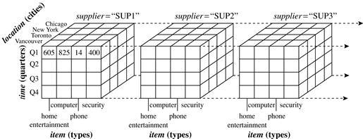
Figure 4.4 A 4-D data cube representation of sales data, according to time, item, location, and supplier. The measure displayed is dollars_sold (in thousands). For improved readability, only some of the cube values are shown.
Tables 4.2 and 4.3 show the data at different degrees of summarization. In the data warehousing research literature, a data cube like those shown in Figures 4.3 and 4.4 is often referred to as a cuboid. Given a set of dimensions, we can generate a cuboid for each of the possible subsets of the given dimensions. The result would form a lattice of cuboids, each showing the data at a different level of summarization, or group-by. The lattice of cuboids is then referred to as a data cube. Figure 4.5 shows a lattice of cuboids forming a data cube for the dimensions time, item, location, and supplier.

Figure 4.5 Lattice of cuboids, making up a 4-D data cube for time, item, location, and supplier. Each cuboid represents a different degree of summarization.
The cuboid that holds the lowest level of summarization is called the base cuboid. For example, the 4-D cuboid in Figure 4.4 is the base cuboid for the given time, item, location, and supplier dimensions. Figure 4.3 is a 3-D (nonbase) cuboid for time, item, and location, summarized for all suppliers. The 0-D cuboid, which holds the highest level of summarization, is called the apex cuboid. In our example, this is the total sales, or dollars_sold, summarized over all four dimensions. The apex cuboid is typically denoted by all.
4.2.2 Stars, Snowflakes, and Fact Constellations: Schemas for Multidimensional Data Models
The entity-relationship data model is commonly used in the design of relational databases, where a database schema consists of a set of entities and the relationships between them. Such a data model is appropriate for online transaction processing. A data warehouse, however, requires a concise, subject-oriented schema that facilitates online data analysis.
The most popular data model for a data warehouse is a multidimensional model, which can exist in the form of a star schema, a snowflake schema, or a fact constellation schema. Let’s look at each of these.
Star schema: The most common modeling paradigm is the star schema, in which the data warehouse contains (1) a large central table (fact table ) containing the bulk of the data, with no redundancy, and (2) a set of smaller attendant tables (dimension tables ), one for each dimension. The schema graph resembles a starburst, with the dimension tables displayed in a radial pattern around the central fact table.

Notice that in the star schema, each dimension is represented by only one table, and each table contains a set of attributes. For example, the location dimension table contains the attribute set {location_key, street, city, province_or_state, country }. This constraint may introduce some redundancy. For example, “Urbana" and “Chicago" are both cities in the state of Illinois, USA. Entries for such cities in the location dimension table will create redundancy among the attributes province_or_state and country; that is, (..., Urbana, IL, USA) and (..., Chicago, IL, USA). Moreover, the attributes within a dimension table may form either a hierarchy (total order) or a lattice (partial order).
Snowflake schema: The snowflake schema is a variant of the star schema model, where some dimension tables are normalized, thereby further splitting the data into additional tables. The resulting schema graph forms a shape similar to a snowflake.
The major difference between the snowflake and star schema models is that the dimension tables of the snowflake model may be kept in normalized form to reduce redundancies. Such a table is easy to maintain and saves storage space. However, this space savings is negligible in comparison to the typical magnitude of the fact table. Furthermore, the snowflake structure can reduce the effectiveness of browsing, since more joins will be needed to execute a query. Consequently, the system performance may be adversely impacted. Hence, although the snowflake schema reduces redundancy, it is not as popular as the star schema in data warehouse design.
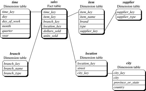
Fact constellation: Sophisticated applications may require multiple fact tables to share dimension tables. This kind of schema can be viewed as a collection of stars, and hence is called a galaxy schema or a fact constellation.

In data warehousing, there is a distinction between a data warehouse and a data mart. A data warehouse collects information about subjects that span the entire organization, such as customers, items, sales, assets, and personnel, and thus its scope is enterprise-wide. For data warehouses, the fact constellation schema is commonly used, since it can model multiple, interrelated subjects. A data mart, on the other hand, is a department subset of the data warehouse that focuses on selected subjects, and thus its scope is department-wide. For data marts, the star or snowflake schema is commonly used, since both are geared toward modeling single subjects, although the star schema is more popular and efficient.
4.2.3 Dimensions: The Role of Concept Hierarchies
A concept hierarchy defines a sequence of mappings from a set of low-level concepts to higher-level, more general concepts. Consider a concept hierarchy for the dimension location. City values for location include Vancouver, Toronto, New York, and Chicago. Each city, however, can be mapped to the province or state to which it belongs. For example, Vancouver can be mapped to British Columbia, and Chicago to Illinois. The provinces and states can in turn be mapped to the country (e.g., Canada or the United States) to which they belong. These mappings form a concept hierarchy for the dimension location, mapping a set of low-level concepts (i.e., cities) to higher-level, more general concepts (i.e., countries). This concept hierarchy is illustrated in Figure 4.9.
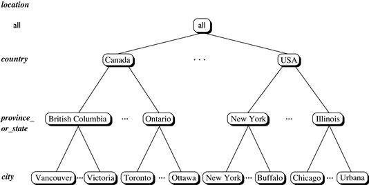
Figure 4.9 A concept hierarchy for location. Due to space limitations, not all of the hierarchy nodes are shown, indicated by ellipses between nodes.
Many concept hierarchies are implicit within the database schema. For example, suppose that the dimension location is described by the attributes number, street, city, province_or_state, zip_code, and country. These attributes are related by a total order, forming a concept hierarchy such as “street < city < province_or_state < country.” This hierarchy is shown in Figure 4.10(a). Alternatively, the attributes of a dimension may be organized in a partial order, forming a lattice. An example of a partial order for the time dimension based on the attributes day, week, month, quarter, and year is “day <{month < quarter; week} < year.”1 This lattice structure is shown in Figure 4.10(b). A concept hierarchy that is a total or partial order among attributes in a database schema is called a schema hierarchy. Concept hierarchies that are common to many applications (e.g., for time) may be predefined in the data mining system. Data mining systems should provide users with the flexibility to tailor predefined hierarchies according to their particular needs. For example, users may want to define a fiscal year starting on April 1 or an academic year starting on September 1.

Figure 4.10 Hierarchical and lattice structures of attributes in warehouse dimensions: (a) a hierarchy for location and (b) a lattice for time.
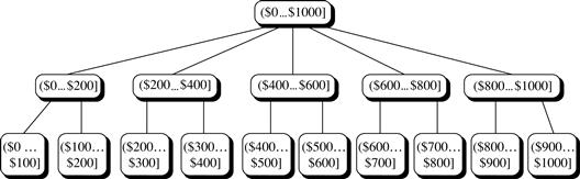
Concept hierarchies may also be defined by discretizing or grouping values for a given dimension or attribute, resulting in a set-grouping hierarchy. A total or partial order can be defined among groups of values. An example of a set-grouping hierarchy is shown in Figure 4.11 for the dimension price, where an interval ($X…$Y] denotes the range from $X (exclusive) to $Y (inclusive).
There may be more than one concept hierarchy for a given attribute or dimension, based on different user viewpoints. For instance, a user may prefer to organize price by defining ranges for inexpensive, moderately_priced, and expensive.
Concept hierarchies may be provided manually by system users, domain experts, or knowledge engineers, or may be automatically generated based on statistical analysis of the data distribution. The automatic generation of concept hierarchies is discussed in Chapter 3 as a preprocessing step in preparation for data mining.
Concept hierarchies allow data to be handled at varying levels of abstraction, as we will see in Section 4.2.4.
4.2.4 Measures: Their Categorization and Computation
“How are measures computed?” To answer this question, we first study how measures can be categorized. Note that a multidimensional point in the data cube space can be defined by a set of dimension–value pairs; for example, ![]() time = “Q1”, location = “Vancouver”, item = “computer”
time = “Q1”, location = “Vancouver”, item = “computer”![]() . A data cube measure is a numeric function that can be evaluated at each point in the data cube space. A measure value is computed for a given point by aggregating the data corresponding to the respective dimension–value pairs defining the given point. We will look at concrete examples of this shortly.
. A data cube measure is a numeric function that can be evaluated at each point in the data cube space. A measure value is computed for a given point by aggregating the data corresponding to the respective dimension–value pairs defining the given point. We will look at concrete examples of this shortly.
Measures can be organized into three categories—distributive, algebraic, and holistic—based on the kind of aggregate functions used.
Distributive: An aggregate function is distributive if it can be computed in a distributed manner as follows. Suppose the data are partitioned into n sets. We apply the function to each partition, resulting in n aggregate values. If the result derived by applying the function to the n aggregate values is the same as that derived by applying the function to the entire data set (without partitioning), the function can be computed in a distributed manner. For example, sum() can be computed for a data cube by first partitioning the cube into a set of subcubes, computing sum() for each subcube, and then summing up the counts obtained for each subcube. Hence, sum() is a distributive aggregate function.
For the same reason, count(), min(), and max() are distributive aggregate functions. By treating the count value of each nonempty base cell as 1 by default, count() of any cell in a cube can be viewed as the sum of the count values of all of its corresponding child cells in its subcube. Thus, count() is distributive. A measure is distributive if it is obtained by applying a distributive aggregate function. Distributive measures can be computed efficiently because of the way the computation can be partitioned.
Algebraic: An aggregate function is algebraic if it can be computed by an algebraic function with M arguments (where M is a bounded positive integer), each of which is obtained by applying a distributive aggregate function. For example, avg() (average) can be computed by sum()/count(), where both sum() and count() are distributive aggregate functions. Similarly, it can be shown that min_N() and max_N() (which find the N minimum and N maximum values, respectively, in a given set) and standard_deviation() are algebraic aggregate functions. A measure is algebraic if it is obtained by applying an algebraic aggregate function.
Holistic: An aggregate function is holistic if there is no constant bound on the storage size needed to describe a subaggregate. That is, there does not exist an algebraic function with M arguments (where M is a constant) that characterizes the computation. Common examples of holistic functions include median(), mode(), and rank(). A measure is holistic if it is obtained by applying a holistic aggregate function.
Most large data cube applications require efficient computation of distributive and algebraic measures. Many efficient techniques for this exist. In contrast, it is difficult to compute holistic measures efficiently. Efficient techniques to approximate the computation of some holistic measures, however, do exist. For example, rather than computing the exact median(), Equation (2.3) of Chapter 2 can be used to estimate the approximate median value for a large data set. In many cases, such techniques are sufficient to overcome the difficulties of efficient computation of holistic measures.
Various methods for computing different measures in data cube construction are discussed in depth in Chapter 5. Notice that most of the current data cube technology confines the measures of multidimensional databases to numeric data. However, measures can also be applied to other kinds of data, such as spatial, multimedia, or text data.
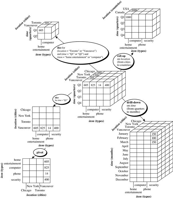
4.2.5 Typical OLAP Operations
“How are concept hierarchies useful in OLAP?” In the multidimensional model, data are organized into multiple dimensions, and each dimension contains multiple levels of abstraction defined by concept hierarchies. This organization provides users with the flexibility to view data from different perspectives. A number of OLAP data cube operations exist to materialize these different views, allowing interactive querying and analysis of the data at hand. Hence, OLAP provides a user-friendly environment for interactive data analysis.
OLAP offers analytical modeling capabilities, including a calculation engine for deriving ratios, variance, and so on, and for computing measures across multiple dimensions. It can generate summarizations, aggregations, and hierarchies at each granularity level and at every dimension intersection. OLAP also supports functional models for forecasting, trend analysis, and statistical analysis. In this context, an OLAP engine is a powerful data analysis tool.
OLAP Systems versus Statistical Databases
Many OLAP systems’ characteristics (e.g., the use of a multidimensional data model and concept hierarchies, the association of measures with dimensions, and the notions of roll-up and drill-down) also exist in earlier work on statistical databases (SDBs). A statistical database is a database system that is designed to support statistical applications. Similarities between the two types of systems are rarely discussed, mainly due to differences in terminology and application domains.
OLAP and SDB systems, however, have distinguishing differences. While SDBs tend to focus on socioeconomic applications, OLAP has been targeted for business applications. Privacy issues regarding concept hierarchies are a major concern for SDBs. For example, given summarized socioeconomic data, it is controversial to allow users to view the corresponding low-level data. Finally, unlike SDBs, OLAP systems are designed for efficiently handling huge amounts of data.
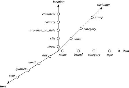
4.2.6 A Starnet Query Model for Querying Multidimensional Databases
The querying of multidimensional databases can be based on a starnet model, which consists of radial lines emanating from a central point, where each line represents a concept hierarchy for a dimension. Each abstraction level in the hierarchy is called a footprint. These represent the granularities available for use by OLAP operations such as drill-down and roll-up.
Example 4.5
Starnet
A starnet query model for the AllElectronics data warehouse is shown in Figure 4.13. This starnet consists of four radial lines, representing concept hierarchies for the dimensions location, customer, item, and time, respectively. Each line consists of footprints representing abstraction levels of the dimension. For example, the time line has four footprints: “day,” “month,” “quarter,” and “year.” A concept hierarchy may involve a single attribute (e.g.,datefor the time hierarchy) or several attributes (e.g., the concept hierarchy for location involves the attributes street, city, province_or_state, and country). In order to examine the item sales at AllElectronics, users can roll up along the time dimension from month to quarter, or, say, drill down along the location dimension from country to city.
Concept hierarchies can be used to generalize data by replacing low-level values (such as “day” for the time dimension) by higher-level abstractions (such as “year”), or to specialize data by replacing higher-level abstractions with lower-level values.