
8.2 Decision Tree Induction
Decision tree induction is the learning of decision trees from class-labeled training tuples. A decision tree is a flowchart-like tree structure, where each internal node (nonleaf node) denotes a test on an attribute, each branch represents an outcome of the test, and each leaf node (or terminal node) holds a class label. The topmost node in a tree is the root node. A typical decision tree is shown in Figure 8.2. It represents the concept buys_computer, that is, it predicts whether a customer at AllElectronics is likely to purchase a computer. Internal nodes are denoted by rectangles, and leaf nodes are denoted by ovals. Some decision tree algorithms produce only binary trees (where each internal node branches to exactly two other nodes), whereas others can produce nonbinary trees.
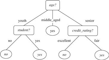
Figure 8.2 A decision tree for the concept buys_computer, indicating whether an AllElectronics customer is likely to purchase a computer. Each internal (nonleaf) node represents a test on an attribute. Each leaf node represents a class (either buys_computer = yes or buys_computer = no).
“How are decision trees used for classification?” Given a tuple, X, for which the associated class label is unknown, the attribute values of the tuple are tested against the decision tree. A path is traced from the root to a leaf node, which holds the class prediction for that tuple. Decision trees can easily be converted to classification rules.
“Why are decision tree classifiers so popular?” The construction of decision tree classifiers does not require any domain knowledge or parameter setting, and therefore is appropriate for exploratory knowledge discovery. Decision trees can handle multidimensional data. Their representation of acquired knowledge in tree form is intuitive and generally easy to assimilate by humans. The learning and classification steps of decision tree induction are simple and fast. In general, decision tree classifiers have good accuracy. However, successful use may depend on the data at hand. Decision tree induction algorithms have been used for classification in many application areas such as medicine, manufacturing and production, financial analysis, astronomy, and molecular biology. Decision trees are the basis of several commercial rule induction systems.
In Section 8.2.1, we describe a basic algorithm for learning decision trees. During tree construction, attribute selection measures are used to select the attribute that best partitions the tuples into distinct classes. Popular measures of attribute selection are given in Section 8.2.2. When decision trees are built, many of the branches may reflect noise or outliers in the training data. Tree pruning attempts to identify and remove such branches, with the goal of improving classification accuracy on unseen data. Tree pruning is described in Section 8.2.3. Scalability issues for the induction of decision trees from large databases are discussed in Section 8.2.4. Section 8.2.5 presents a visual mining approach to decision tree induction.
8.2.1 Decision Tree Induction
During the late 1970s and early 1980s, J. Ross Quinlan, a researcher in machine learning, developed a decision tree algorithm known as ID3 (Iterative Dichotomiser). This work expanded on earlier work on concept learning systems, described by E. B. Hunt, J. Marin, and P. T. Stone. Quinlan later presented C4.5 (a successor of ID3), which became a benchmark to which newer supervised learning algorithms are often compared. In 1984, a group of statisticians (L. Breiman, J. Friedman, R. Olshen, and C. Stone) published the book Classification and Regression Trees (CART), which described the generation of binary decision trees. ID3 and CART were invented independently of one another at around the same time, yet follow a similar approach for learning decision trees from training tuples. These two cornerstone algorithms spawned a flurry of work on decision tree induction.
ID3, C4.5, and CART adopt a greedy (i.e., nonbacktracking) approach in which decision trees are constructed in a top-down recursive divide-and-conquer manner. Most algorithms for decision tree induction also follow a top-down approach, which starts with a training set of tuples and their associated class labels. The training set is recursively partitioned into smaller subsets as the tree is being built. A basic decision tree algorithm is summarized in Figure 8.3. At first glance, the algorithm may appear long, but fear not! It is quite straightforward. The strategy is as follows.
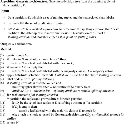
■ The algorithm is called with three parameters: D, attribute_list, and Attribute_ selection_method. We refer to D as a data partition. Initially, it is the complete set of training tuples and their associated class labels. The parameter attribute_list is a list of attributes describing the tuples. Attribute_selection_method specifies a heuristic procedure for selecting the attribute that “best” discriminates the given tuples according to class. This procedure employs an attribute selection measure such as information gain or the Gini index. Whether the tree is strictly binary is generally driven by the attribute selection measure. Some attribute selection measures, such as the Gini index, enforce the resulting tree to be binary. Others, like information gain, do not, therein allowing multiway splits (i.e., two or more branches to be grown from a node).
■ The tree starts as a single node, N, representing the training tuples in D (step 1).3
■ If the tuples in D are all of the same class, then node N becomes a leaf and is labeled with that class (steps 2 and 3). Note that steps 4 and 5 are terminating conditions. All terminating conditions are explained at the end of the algorithm.
■ Otherwise, the algorithm calls Attribute_selection_method to determine the splitting criterion. The splitting criterion tells us which attribute to test at node N by determining the “best” way to separate or partition the tuples in D into individual classes (step 6). The splitting criterion also tells us which branches to grow from node N with respect to the outcomes of the chosen test. More specifically, the splitting criterion indicates the splitting attribute and may also indicate either a split-point or a splitting subset. The splitting criterion is determined so that, ideally, the resulting partitions at each branch are as “pure” as possible. A partition is pure if all the tuples in it belong to the same class. In other words, if we split up the tuples in D according to the mutually exclusive outcomes of the splitting criterion, we hope for the resulting partitions to be as pure as possible.
■ The node N is labeled with the splitting criterion, which serves as a test at the node (step 7). A branch is grown from node N for each of the outcomes of the splitting criterion. The tuples in D are partitioned accordingly (steps 10 to 11). There are three possible scenarios, as illustrated in Figure 8.4. Let A be the splitting attribute. A has v distinct values, {![]() }, based on the training data.
}, based on the training data.
1. A is discrete-valued: In this case, the outcomes of the test at node N correspond directly to the known values of A. A branch is created for each known value, aj, of A and labeled with that value (Figure 8.4a). Partition Dj is the subset of class-labeled tuples in D having value aj of A. Because all the tuples in a given partition have the same value for A, A need not be considered in any future partitioning of the tuples. Therefore, it is removed from attribute_list (steps 8 and 9).
2. A is continuous-valued: In this case, the test at node N has two possible outcomes, corresponding to the conditions ![]() split_point and
split_point and ![]() split_point, respectively, where split_point is the split-point returned by Attribute_selection_method as part of the splitting criterion. (In practice, the split-point, a, is often taken as the midpoint of two known adjacent values of A and therefore may not actually be a preexisting value of A from the training data.) Two branches are grown from N and labeled according to the previous outcomes (Figure 8.4b). The tuples are partitioned such that D1 holds the subset of class-labeled tuples in D for which
split_point, respectively, where split_point is the split-point returned by Attribute_selection_method as part of the splitting criterion. (In practice, the split-point, a, is often taken as the midpoint of two known adjacent values of A and therefore may not actually be a preexisting value of A from the training data.) Two branches are grown from N and labeled according to the previous outcomes (Figure 8.4b). The tuples are partitioned such that D1 holds the subset of class-labeled tuples in D for which ![]() split_point, while D2 holds the rest.
split_point, while D2 holds the rest.
3. A is discrete-valued and a binary tree must be produced (as dictated by the attribute selection measure or algorithm being used): The test at node N is of the form “![]() ?,” where SA is the splitting subset for A, returned by Attribute_selection_method as part of the splitting criterion. It is a subset of the known values of A. If a given tuple has value aj of A and if
?,” where SA is the splitting subset for A, returned by Attribute_selection_method as part of the splitting criterion. It is a subset of the known values of A. If a given tuple has value aj of A and if ![]() , then the test at node N is satisfied. Two branches are grown from N (Figure 8.4c). By convention, the left branch out of N is labeled yes so that D1 corresponds to the subset of class-labeled tuples in D that satisfy the test. The right branch out of N is labeled no so that D2 corresponds to the subset of class-labeled tuples from D that do not satisfy the test.
, then the test at node N is satisfied. Two branches are grown from N (Figure 8.4c). By convention, the left branch out of N is labeled yes so that D1 corresponds to the subset of class-labeled tuples in D that satisfy the test. The right branch out of N is labeled no so that D2 corresponds to the subset of class-labeled tuples from D that do not satisfy the test.

Figure 8.4 This figure shows three possibilities for partitioning tuples based on the splitting criterion, each with examples. Let A be the splitting attribute. (a) If A is discrete-valued, then one branch is grown for each known value of A. (b) If A is continuous-valued, then two branches are grown, corresponding to A ≤ split_point and A > split_point. (c) If A is discrete-valued and a binary tree must be produced, then the test is of the form A ∈ SA, where SA is the splitting subset for A.
■ The algorithm uses the same process recursively to form a decision tree for the tuples at each resulting partition, Dj, of D (step 14).
■ The recursive partitioning stops only when any one of the following terminating conditions is true:
1. All the tuples in partition D (represented at node N) belong to the same class (steps 2 and 3).
2. There are no remaining attributes on which the tuples may be further partitioned (step 4). In this case, majority voting is employed (step 5). This involves converting node N into a leaf and labeling it with the most common class in D. Alternatively, the class distribution of the node tuples may be stored.
3. There are no tuples for a given branch, that is, a partition Dj is empty (step 12). In this case, a leaf is created with the majority class in D (step 13).
The computational complexity of the algorithm given training set D is ![]() , where n is the number of attributes describing the tuples in D and
, where n is the number of attributes describing the tuples in D and ![]() is the number of training tuples in D. This means that the computational cost of growing a tree grows at most
is the number of training tuples in D. This means that the computational cost of growing a tree grows at most ![]() with
with ![]() tuples. The proof is left as an exercise for the reader.
tuples. The proof is left as an exercise for the reader.
Incremental versions of decision tree induction have also been proposed. When given new training data, these restructure the decision tree acquired from learning on previous training data, rather than relearning a new tree from scratch.
Differences in decision tree algorithms include how the attributes are selected in creating the tree (Section 8.2.2) and the mechanisms used for pruning (Section 8.2.3). The basic algorithm described earlier requires one pass over the training tuples in D for each level of the tree. This can lead to long training times and lack of available memory when dealing with large databases. Improvements regarding the scalability of decision tree induction are discussed in Section 8.2.4. Section 8.2.5 presents a visual interactive approach to decision tree construction. A discussion of strategies for extracting rules from decision trees is given in Section 8.4.2 regarding rule-based classification.
8.2.2 Attribute Selection Measures
An attribute selection measure is a heuristic for selecting the splitting criterion that “best” separates a given data partition, D, of class-labeled training tuples into individual classes. If we were to split D into smaller partitions according to the outcomes of the splitting criterion, ideally each partition would be pure (i.e., all the tuples that fall into a given partition would belong to the same class). Conceptually, the “best” splitting criterion is the one that most closely results in such a scenario. Attribute selection measures are also known as splitting rules because they determine how the tuples at a given node are to be split.
The attribute selection measure provides a ranking for each attribute describing the given training tuples. The attribute having the best score for the measure4 is chosen as the splitting attribute for the given tuples. If the splitting attribute is continuous-valued or if we are restricted to binary trees, then, respectively, either a split point or a splitting subset must also be determined as part of the splitting criterion. The tree node created for partition D is labeled with the splitting criterion, branches are grown for each outcome of the criterion, and the tuples are partitioned accordingly. This section describes three popular attribute selection measures—information gain, gain ratio, and Gini index.
The notation used herein is as follows. Let D, the data partition, be a training set of class-labeled tuples. Suppose the class label attribute has m distinct values defining m distinct classes, Ci (for ![]() ). Let
). Let ![]() be the set of tuples of class Ci in D. Let
be the set of tuples of class Ci in D. Let ![]() and
and ![]() denote the number of tuples in D and
denote the number of tuples in D and ![]() , respectively.
, respectively.
Information Gain
ID3 uses information gain as its attribute selection measure. This measure is based on pioneering work by Claude Shannon on information theory, which studied the value or “information content” of messages. Let node N represent or hold the tuples of partition D. The attribute with the highest information gain is chosen as the splitting attribute for node N. This attribute minimizes the information needed to classify the tuples in the resulting partitions and reflects the least randomness or “impurity” in these partitions. Such an approach minimizes the expected number of tests needed to classify a given tuple and guarantees that a simple (but not necessarily the simplest) tree is found.
The expected information needed to classify a tuple in D is given by
![]() (8.1)
(8.1)
where pi is the nonzero probability that an arbitrary tuple in D belongs to class Ci and is estimated by ![]() /
/![]() . A log function to the base 2 is used, because the information is encoded in bits. Info (D) is just the average amount of information needed to identify the class label of a tuple in D. Note that, at this point, the information we have is based solely on the proportions of tuples of each class. Info (D) is also known as the entropy of D.
. A log function to the base 2 is used, because the information is encoded in bits. Info (D) is just the average amount of information needed to identify the class label of a tuple in D. Note that, at this point, the information we have is based solely on the proportions of tuples of each class. Info (D) is also known as the entropy of D.
Now, suppose we were to partition the tuples in D on some attribute A having v distinct values, {![]() }, as observed from the training data. If A is discrete-valued, these values correspond directly to the v outcomes of a test on A. Attribute A can be used to split D into v partitions or subsets, {
}, as observed from the training data. If A is discrete-valued, these values correspond directly to the v outcomes of a test on A. Attribute A can be used to split D into v partitions or subsets, {![]() }, where Dj contains those tuples in D that have outcome aj of A. These partitions would correspond to the branches grown from node N. Ideally, we would like this partitioning to produce an exact classification of the tuples. That is, we would like for each partition to be pure. However, it is quite likely that the partitions will be impure (e.g., where a partition may contain a collection of tuples from different classes rather than from a single class).
}, where Dj contains those tuples in D that have outcome aj of A. These partitions would correspond to the branches grown from node N. Ideally, we would like this partitioning to produce an exact classification of the tuples. That is, we would like for each partition to be pure. However, it is quite likely that the partitions will be impure (e.g., where a partition may contain a collection of tuples from different classes rather than from a single class).
How much more information would we still need (after the partitioning) to arrive at an exact classification? This amount is measured by
![]() (8.2)
(8.2)
The term ![]() acts as the weight of the j th partition.
acts as the weight of the j th partition. ![]() is the expected information required to classify a tuple from D based on the partitioning by A. The smaller the expected information (still) required, the greater the purity of the partitions.
is the expected information required to classify a tuple from D based on the partitioning by A. The smaller the expected information (still) required, the greater the purity of the partitions.
Information gain is defined as the difference between the original information requirement (i.e., based on just the proportion of classes) and the new requirement (i.e., obtained after partitioning on A). That is,
![]() (8.3)
(8.3)
In other words, Gain(A) tells us how much would be gained by branching on A. It is the expected reduction in the information requirement caused by knowing the value of A. The attribute A with the highest information gain, Gain(A), is chosen as the splitting attribute at node N. This is equivalent to saying that we want to partition on the attribute A that would do the “best classification,” so that the amount of information still required to finish classifying the tuples is minimal (i.e., minimum ![]() ).
).
Example 8.1
Induction of a decision tree using information gain
Table 8.1 presents a training set, D, of class-labeled tuples randomly selected from the AllElectronics customer database. (The data are adapted from Quinlan [Qui86]. In this example, each attribute is discrete-valued. Continuous-valued attributes have been generalized.) The class label attribute, buys_computer, has two distinct values (namely, {yes, no}); therefore, there are two distinct classes (i.e., ![]() ). Let class C1 correspond to yes and class C2 correspond to no. There are nine tuples of class yes and five tuples of class no. A (root) node N is created for the tuples in D. To find the splitting criterion for these tuples, we must compute the information gain of each attribute. We first use Eq. (8.1) to compute the expected information needed to classify a tuple in D:
). Let class C1 correspond to yes and class C2 correspond to no. There are nine tuples of class yes and five tuples of class no. A (root) node N is created for the tuples in D. To find the splitting criterion for these tuples, we must compute the information gain of each attribute. We first use Eq. (8.1) to compute the expected information needed to classify a tuple in D:
![]()
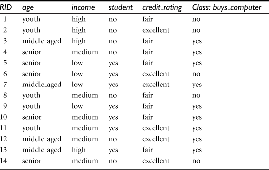
Next, we need to compute the expected information requirement for each attribute. Let’s start with the attribute age. We need to look at the distribution of yes and no tuples for each category of age. For the age category “youth,” there are two yes tuples and three no tuples. For the category “middle_aged,” there are four yes tuples and zero no tuples. For the category “senior,” there are three yes tuples and two no tuples. Using Eq. (8.2), the expected information needed to classify a tuple in D if the tuples are partitioned according to age is
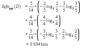
Hence, the gain in information from such a partitioning would be
![]()
Similarly, we can compute ![]() bits,
bits, ![]() bits, and
bits, and ![]() bits. Because age has the highest information gain among the attributes, it is selected as the splitting attribute. Node N is labeled with age, and branches are grown for each of the attribute’s values. The tuples are then partitioned accordingly, as shown in Figure 8.5. Notice that the tuples falling into the partition for age = middle_aged all belong to the same class. Because they all belong to class “yes,” a leaf should therefore be created at the end of this branch and labeled “yes.” The final decision tree returned by the algorithm was shown earlier in Figure 8.2.
bits. Because age has the highest information gain among the attributes, it is selected as the splitting attribute. Node N is labeled with age, and branches are grown for each of the attribute’s values. The tuples are then partitioned accordingly, as shown in Figure 8.5. Notice that the tuples falling into the partition for age = middle_aged all belong to the same class. Because they all belong to class “yes,” a leaf should therefore be created at the end of this branch and labeled “yes.” The final decision tree returned by the algorithm was shown earlier in Figure 8.2.

Figure 8.5 The attribute age has the highest information gain and therefore becomes the splitting attribute at the root node of the decision tree. Branches are grown for each outcome of age. The tuples are shown partitioned accordingly.
“But how can we compute the information gain of an attribute that is continuous-valued, unlike in the example?” Suppose, instead, that we have an attribute A that is continuous-valued, rather than discrete-valued. (For example, suppose that instead of the discretized version of age from the example, we have the raw values for this attribute.) For such a scenario, we must determine the “best” split-point for A, where the split-point is a threshold on A.
We first sort the values of A in increasing order. Typically, the midpoint between each pair of adjacent values is considered as a possible split-point. Therefore, given v values of A, then ![]() possible splits are evaluated. For example, the midpoint between the values ai and
possible splits are evaluated. For example, the midpoint between the values ai and ![]() of A is
of A is
![]() (8.4)
(8.4)
If the values of A are sorted in advance, then determining the best split for A requires only one pass through the values. For each possible split-point for A, we evaluate ![]() , where the number of partitions is two, that is,
, where the number of partitions is two, that is, ![]() (or
(or ![]() ) in Eq. (8.2). The point with the minimum expected information requirement for A is selected as the split_point for A. D1 is the set of tuples in D satisfying
) in Eq. (8.2). The point with the minimum expected information requirement for A is selected as the split_point for A. D1 is the set of tuples in D satisfying ![]() , and D2 is the set of tuples in D satisfying
, and D2 is the set of tuples in D satisfying ![]() .
.
Gain Ratio
The information gain measure is biased toward tests with many outcomes. That is, it prefers to select attributes having a large number of values. For example, consider an attribute that acts as a unique identifier such as product_ID. A split on product_ID would result in a large number of partitions (as many as there are values), each one containing just one tuple. Because each partition is pure, the information required to classify data set D based on this partitioning would be ![]() . Therefore, the information gained by partitioning on this attribute is maximal. Clearly, such a partitioning is useless for classification.
. Therefore, the information gained by partitioning on this attribute is maximal. Clearly, such a partitioning is useless for classification.
C4.5, a successor of ID3, uses an extension to information gain known as gain ratio, which attempts to overcome this bias. It applies a kind of normalization to information gain using a “split information” value defined analogously with ![]() as
as
![]() (8.5)
(8.5)
This value represents the potential information generated by splitting the training data set, D, into v partitions, corresponding to the v outcomes of a test on attribute A. Note that, for each outcome, it considers the number of tuples having that outcome with respect to the total number of tuples in D. It differs from information gain, which measures the information with respect to classification that is acquired based on the same partitioning. The gain ratio is defined as
![]() (8.6)
(8.6)
The attribute with the maximum gain ratio is selected as the splitting attribute. Note, however, that as the split information approaches 0, the ratio becomes unstable. A constraint is added to avoid this, whereby the information gain of the test selected must be large—at least as great as the average gain over all tests examined.
Example 8.2
Computation of gain ratio for the attribute income
A test on income splits the data of Table 8.1 into three partitions, namely low, medium, and high, containing four, six, and four tuples, respectively. To compute the gain ratio of income, we first use Eq. (8.5) to obtain

From Example 8.1, we have Gain(income) = 0.029. Therefore, GainRatio (income) = 0.029/1.557 = 0.019.
Gini Index
The Gini index is used in CART. Using the notation previously described, the Gini index measures the impurity of D, a data partition or set of training tuples, as
![]() (8.7)
(8.7)
where pi is the probability that a tuple in D belongs to class Ci and is estimated by ![]() /
/![]() . The sum is computed over m classes.
. The sum is computed over m classes.
The Gini index considers a binary split for each attribute. Let’s first consider the case where A is a discrete-valued attribute having v distinct values, {![]() }, occurring in D. To determine the best binary split on A, we examine all the possible subsets that can be formed using known values of A. Each subset, SA, can be considered as a binary test for attribute A of the form “
}, occurring in D. To determine the best binary split on A, we examine all the possible subsets that can be formed using known values of A. Each subset, SA, can be considered as a binary test for attribute A of the form “![]() ?” Given a tuple, this test is satisfied if the value of A for the tuple is among the values listed in SA. If A has v possible values, then there are
?” Given a tuple, this test is satisfied if the value of A for the tuple is among the values listed in SA. If A has v possible values, then there are ![]() possible subsets. For example, if income has three possible values, namely {low, medium, high}, then the possible subsets are {low, medium, high}, {low, medium}, {low, high}, {medium, high}, {low}, {medium}, {high}, and {}. We exclude the power set, {low, medium, high}, and the empty set from consideration since, conceptually, they do not represent a split. Therefore, there are (2v − 2)/2 possible ways to form two partitions of the data, D, based on a binary split on A.
possible subsets. For example, if income has three possible values, namely {low, medium, high}, then the possible subsets are {low, medium, high}, {low, medium}, {low, high}, {medium, high}, {low}, {medium}, {high}, and {}. We exclude the power set, {low, medium, high}, and the empty set from consideration since, conceptually, they do not represent a split. Therefore, there are (2v − 2)/2 possible ways to form two partitions of the data, D, based on a binary split on A.
When considering a binary split, we compute a weighted sum of the impurity of each resulting partition. For example, if a binary split on A partitions D into D1 and D2, the Gini index of D given that partitioning is
![]() (8.8)
(8.8)
For each attribute, each of the possible binary splits is considered. For a discrete-valued attribute, the subset that gives the minimum Gini index for that attribute is selected as its splitting subset.
For continuous-valued attributes, each possible split-point must be considered. The strategy is similar to that described earlier for information gain, where the midpoint between each pair of (sorted) adjacent values is taken as a possible split-point. The point giving the minimum Gini index for a given (continuous-valued) attribute is taken as the split-point of that attribute. Recall that for a possible split-point of A, D1 is the set of tuples in D satisfying ![]() , and D2 is the set of tuples in D satisfying
, and D2 is the set of tuples in D satisfying ![]() .
.
The reduction in impurity that would be incurred by a binary split on a discrete- or continuous-valued attribute A is
![]() (8.9)
(8.9)
The attribute that maximizes the reduction in impurity (or, equivalently, has the minimum Gini index) is selected as the splitting attribute. This attribute and either its splitting subset (for a discrete-valued splitting attribute) or split-point (for a continuous-valued splitting attribute) together form the splitting criterion.
Example 8.3
Induction of a decision tree using the Gini index
Let D be the training data shown earlier in Table 8.1, where there are nine tuples belonging to the class buys_computer = yes and the remaining five tuples belong to the class buys_computer = no. A (root) node N is created for the tuples in D. We first use Eq. (8.7) for the Gini index to compute the impurity of D:
![]()
To find the splitting criterion for the tuples in D, we need to compute the Gini index for each attribute. Let’s start with the attribute income and consider each of the possible splitting subsets. Consider the subset {low, medium}. This would result in 10 tuples in partition D1 satisfying the condition “income ![]() {low, medium}.” The remaining four tuples of D would be assigned to partition D2. The Gini index value computed based on this partitioning is
{low, medium}.” The remaining four tuples of D would be assigned to partition D2. The Gini index value computed based on this partitioning is

Similarly, the Gini index values for splits on the remaining subsets are 0.458 (for the subsets {low, high} and {medium}) and 0.450 (for the subsets {medium, high} and {low}). Therefore, the best binary split for attribute income is on {low, medium} (or {high}) because it minimizes the Gini index. Evaluating age, we obtain {youth, senior} (or {middle_aged}) as the best split for age with a Gini index of 0.375; the attributes student and credit_rating are both binary, with Gini index values of 0.367 and 0.429, respectively.
The attribute age and splitting subset {youth, senior} therefore give the minimum Gini index overall, with a reduction in impurity of ![]() . The binary split “age
. The binary split “age ![]() {youth, senior?}” results in the maximum reduction in impurity of the tuples in D and is returned as the splitting criterion. Node N is labeled with the criterion, two branches are grown from it, and the tuples are partitioned accordingly.
{youth, senior?}” results in the maximum reduction in impurity of the tuples in D and is returned as the splitting criterion. Node N is labeled with the criterion, two branches are grown from it, and the tuples are partitioned accordingly.
Other Attribute Selection Measures
This section on attribute selection measures was not intended to be exhaustive. We have shown three measures that are commonly used for building decision trees. These measures are not without their biases. Information gain, as we saw, is biased toward multivalued attributes. Although the gain ratio adjusts for this bias, it tends to prefer unbalanced splits in which one partition is much smaller than the others. The Gini index is biased toward multivalued attributes and has difficulty when the number of classes is large. It also tends to favor tests that result in equal-size partitions and purity in both partitions. Although biased, these measures give reasonably good results in practice.
Many other attribute selection measures have been proposed. CHAID, a decision tree algorithm that is popular in marketing, uses an attribute selection measure that is based on the statistical ![]() test for independence. Other measures include C-SEP (which performs better than information gain and the Gini index in certain cases) and G-statistic (an information theoretic measure that is a close approximation to
test for independence. Other measures include C-SEP (which performs better than information gain and the Gini index in certain cases) and G-statistic (an information theoretic measure that is a close approximation to ![]() distribution).
distribution).
Attribute selection measures based on the Minimum Description Length (MDL) principle have the least bias toward multivalued attributes. MDL-based measures use encoding techniques to define the “best” decision tree as the one that requires the fewest number of bits to both (1) encode the tree and (2) encode the exceptions to the tree (i.e., cases that are not correctly classified by the tree). Its main idea is that the simplest of solutions is preferred.
Other attribute selection measures consider multivariate splits (i.e., where the partitioning of tuples is based on a combination of attributes, rather than on a single attribute). The CART system, for example, can find multivariate splits based on a linear combination of attributes. Multivariate splits are a form of attribute (or feature) construction, where new attributes are created based on the existing ones. (Attribute construction was also discussed in Chapter 3, as a form of data transformation.) These other measures mentioned here are beyond the scope of this book. Additional references are given in the bibliographic notes at the end of this chapter (Section 8.9).
“Which attribute selection measure is the best?” All measures have some bias. It has been shown that the time complexity of decision tree induction generally increases exponentially with tree height. Hence, measures that tend to produce shallower trees (e.g., with multiway rather than binary splits, and that favor more balanced splits) may be preferred. However, some studies have found that shallow trees tend to have a large number of leaves and higher error rates. Despite several comparative studies, no one attribute selection measure has been found to be significantly superior to others. Most measures give quite good results.
8.2.3 Tree Pruning
When a decision tree is built, many of the branches will reflect anomalies in the training data due to noise or outliers. Tree pruning methods address this problem of overfitting the data. Such methods typically use statistical measures to remove the least-reliable branches. An unpruned tree and a pruned version of it are shown in Figure 8.6. Pruned trees tend to be smaller and less complex and, thus, easier to comprehend. They are usually faster and better at correctly classifying independent test data (i.e., of previously unseen tuples) than unpruned trees.

“How does tree pruning work?” There are two common approaches to tree pruning: prepruning and postpruning.
In the prepruning approach, a tree is “pruned” by halting its construction early (e.g., by deciding not to further split or partition the subset of training tuples at a given node). Upon halting, the node becomes a leaf. The leaf may hold the most frequent class among the subset tuples or the probability distribution of those tuples.
When constructing a tree, measures such as statistical significance, information gain, Gini index, and so on, can be used to assess the goodness of a split. If partitioning the tuples at a node would result in a split that falls below a prespecified threshold, then further partitioning of the given subset is halted. There are difficulties, however, in choosing an appropriate threshold. High thresholds could result in oversimplified trees, whereas low thresholds could result in very little simplification.
The second and more common approach is postpruning, which removes subtrees from a “fully grown” tree. A subtree at a given node is pruned by removing its branches and replacing it with a leaf. The leaf is labeled with the most frequent class among the subtree being replaced. For example, notice the subtree at node “A3?” in the unpruned tree of Figure 8.6. Suppose that the most common class within this subtree is “class B.” In the pruned version of the tree, the subtree in question is pruned by replacing it with the leaf “class B.”
The cost complexity pruning algorithm used in CART is an example of the postpruning approach. This approach considers the cost complexity of a tree to be a function of the number of leaves in the tree and the error rate of the tree (where the error rate is the percentage of tuples misclassified by the tree). It starts from the bottom of the tree. For each internal node, N, it computes the cost complexity of the subtree at N, and the cost complexity of the subtree at N if it were to be pruned (i.e., replaced by a leaf node). The two values are compared. If pruning the subtree at node N would result in a smaller cost complexity, then the subtree is pruned. Otherwise, it is kept.
A pruning set of class-labeled tuples is used to estimate cost complexity. This set is independent of the training set used to build the unpruned tree and of any test set used for accuracy estimation. The algorithm generates a set of progressively pruned trees. In general, the smallest decision tree that minimizes the cost complexity is preferred.
C4.5 uses a method called pessimistic pruning, which is similar to the cost complexity method in that it also uses error rate estimates to make decisions regarding subtree pruning. Pessimistic pruning, however, does not require the use of a prune set. Instead, it uses the training set to estimate error rates. Recall that an estimate of accuracy or error based on the training set is overly optimistic and, therefore, strongly biased. The pessimistic pruning method therefore adjusts the error rates obtained from the training set by adding a penalty, so as to counter the bias incurred.
Rather than pruning trees based on estimated error rates, we can prune trees based on the number of bits required to encode them. The “best” pruned tree is the one that minimizes the number of encoding bits. This method adopts the MDL principle, which was briefly introduced in Section 8.2.2. The basic idea is that the simplest solution is preferred. Unlike cost complexity pruning, it does not require an independent set of tuples.
Alternatively, prepruning and postpruning may be interleaved for a combined approach. Postpruning requires more computation than prepruning, yet generally leads to a more reliable tree. No single pruning method has been found to be superior over all others. Although some pruning methods do depend on the availability of additional data for pruning, this is usually not a concern when dealing with large databases.
Although pruned trees tend to be more compact than their unpruned counterparts, they may still be rather large and complex. Decision trees can suffer from repetition and replication (Figure 8.7), making them overwhelming to interpret. Repetition occurs when an attribute is repeatedly tested along a given branch of the tree (e.g., “age < 60?,” followed by ”age < 45?,” and so on). In replication, duplicate subtrees exist within the tree. These situations can impede the accuracy and comprehensibility of a decision tree. The use of multivariate splits (splits based on a combination of attributes) can prevent these problems. Another approach is to use a different form of knowledge representation, such as rules, instead of decision trees. This is described in Section 8.4.2, which shows how a rule-based classifier can be constructed by extracting IF-THEN rules from a decision tree.

8.2.4 Scalability and Decision Tree Induction
“What if D, the disk-resident training set of class-labeled tuples, does not fit in memory? In other words, how scalable is decision tree induction?” The efficiency of existing decision tree algorithms, such as ID3, C4.5, and CART, has been well established for relatively small data sets. Efficiency becomes an issue of concern when these algorithms are applied to the mining of very large real-world databases. The pioneering decision tree algorithms that we have discussed so far have the restriction that the training tuples should reside in memory.
In data mining applications, very large training sets of millions of tuples are common. Most often, the training data will not fit in memory! Therefore, decision tree construction becomes inefficient due to swapping of the training tuples in and out of main and cache memories. More scalable approaches, capable of handling training data that are too large to fit in memory, are required. Earlier strategies to “save space” included discretizing continuous-valued attributes and sampling data at each node. These techniques, however, still assume that the training set can fit in memory.
Several scalable decision tree induction methods have been introduced in recent studies. RainForest, for example, adapts to the amount of main memory available and applies to any decision tree induction algorithm. The method maintains an AVC-set (where “AVC” stands for “Attribute-Value, Classlabel”) for each attribute, at each tree node, describing the training tuples at the node. The AVC-set of an attribute A at node N gives the class label counts for each value of A for the tuples at N. Figure 8.8 shows AVC-sets for the tuple data of Table 8.1. The set of all AVC-sets at a node N is the AVC-group of N. The size of an AVC-set for attribute A at node N depends only on the number of distinct values of A and the number of classes in the set of tuples at N. Typically, this size should fit in memory, even for real-world data. RainForest also has techniques, however, for handling the case where the AVC-group does not fit in memory. Therefore, the method has high scalability for decision tree induction in very large data sets.
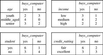
Figure 8.8 The use of data structures to hold aggregate information regarding the training data (e.g., these AVC-sets describing Table 8.1’s data) are one approach to improving the scalability of decision tree induction.
BOAT (Bootstrapped Optimistic Algorithm for Tree construction) is a decision tree algorithm that takes a completely different approach to scalability—it is not based on the use of any special data structures. Instead, it uses a statistical technique known as “bootstrapping” (Section 8.5.4) to create several smaller samples (or subsets) of the given training data, each of which fits in memory. Each subset is used to construct a tree, resulting in several trees. The trees are examined and used to construct a new tree, ![]() , that turns out to be “very close” to the tree that would have been generated if all the original training data had fit in memory.
, that turns out to be “very close” to the tree that would have been generated if all the original training data had fit in memory.
BOAT can use any attribute selection measure that selects binary splits and that is based on the notion of purity of partitions such as the Gini index. BOAT uses a lower bound on the attribute selection measure to detect if this “very good” tree, ![]() , is different from the “real” tree, T, that would have been generated using all of the data. It refines
, is different from the “real” tree, T, that would have been generated using all of the data. It refines ![]() to arrive at T.
to arrive at T.
BOAT usually requires only two scans of D. This is quite an improvement, even in comparison to traditional decision tree algorithms (e.g., the basic algorithm in Figure 8.3), which require one scan per tree level! BOAT was found to be two to three times faster than RainForest, while constructing exactly the same tree. An additional advantage of BOAT is that it can be used for incremental updates. That is, BOAT can take new insertions and deletions for the training data and update the decision tree to reflect these changes, without having to reconstruct the tree from scratch.
8.2.5 Visual Mining for Decision Tree Induction
“Are there any interactive approaches to decision tree induction that allow us to visualize the data and the tree as it is being constructed? Can we use any knowledge of our data to help in building the tree?” In this section, you will learn about an approach to decision tree induction that supports these options. Perception-based classification (PBC) is an interactive approach based on multidimensional visualization techniques and allows the user to incorporate background knowledge about the data when building a decision tree. By visually interacting with the data, the user is also likely to develop a deeper understanding of the data. The resulting trees tend to be smaller than those built using traditional decision tree induction methods and so are easier to interpret, while achieving about the same accuracy.
“How can the data be visualized to support interactive decision tree construction?” PBC uses a pixel-oriented approach to view multidimensional data with its class label information. The circle segments approach is adapted, which maps d-dimensional data objects to a circle that is partitioned into d segments, each representing one attribute (Section 2.3.1). Here, an attribute value of a data object is mapped to one colored pixel, reflecting the object’s class label. This mapping is done for each attribute–value pair of each data object. Sorting is done for each attribute to determine the arrangement order within a segment. For example, attribute values within a given segment may be organized so as to display homogeneous (with respect to class label) regions within the same attribute value. The amount of training data that can be visualized at one time is approximately determined by the product of the number of attributes and the number of data objects.
The PBC system displays a split screen, consisting of a Data Interaction window and a Knowledge Interaction window (Figure 8.9). The Data Interaction window displays the circle segments of the data under examination, while the Knowledge Interaction window displays the decision tree constructed so far. Initially, the complete training set is visualized in the Data Interaction window, while the Knowledge Interaction window displays an empty decision tree.

Figure 8.9 A screenshot of PBC, a system for interactive decision tree construction. Multidimensional training data are viewed as circle segments in the Data Interaction window (left). The Knowledge Interaction window (right) displays the current decision tree. Source: From Ankerst, Elsen, Ester, and Kriegel [AEEK99].
Traditional decision tree algorithms allow only binary splits for numeric attributes. PBC, however, allows the user to specify multiple split-points, resulting in multiple branches to be grown from a single tree node.
A tree is interactively constructed as follows. The user visualizes the multidimensional data in the Data Interaction window and selects a splitting attribute and one or more split-points. The current decision tree in the Knowledge Interaction window is expanded. The user selects a node of the decision tree. The user may either assign a class label to the node (which makes the node a leaf) or request the visualization of the training data corresponding to the node. This leads to a new visualization of every attribute except the ones used for splitting criteria on the same path from the root. The interactive process continues until a class has been assigned to each leaf of the decision tree.
The trees constructed with PBC were compared with trees generated by the CART, C4.5, and SPRINT algorithms from various data sets. The trees created with PBC were of comparable accuracy with the tree from the algorithmic approaches, yet were significantly smaller and, thus, easier to understand. Users can use their domain knowledge in building a decision tree, but also gain a deeper understanding of their data during the construction process.