
10.3 Hierarchical Methods
While partitioning methods meet the basic clustering requirement of organizing a set of objects into a number of exclusive groups, in some situations we may want to partition our data into groups at different levels such as in a hierarchy. A hierarchical clustering method works by grouping data objects into a hierarchy or “tree” of clusters.
Representing data objects in the form of a hierarchy is useful for data summarization and visualization. For example, as the manager of human resources at AllElectronics, you may organize your employees into major groups such as executives, managers, and staff. You can further partition these groups into smaller subgroups. For instance, the general group of staff can be further divided into subgroups of senior officers, officers, and trainees. All these groups form a hierarchy. We can easily summarize or characterize the data that are organized into a hierarchy, which can be used to find, say, the average salary of managers and of officers.
Consider handwritten character recognition as another example. A set of handwriting samples may be first partitioned into general groups where each group corresponds to a unique character. Some groups can be further partitioned into subgroups since a character may be written in multiple substantially different ways. If necessary, the hierarchical partitioning can be continued recursively until a desired granularity is reached.
In the previous examples, although we partitioned the data hierarchically, we did not assume that the data have a hierarchical structure (e.g., managers are at the same level in our AllElectronics hierarchy as staff). Our use of a hierarchy here is just to summarize and represent the underlying data in a compressed way. Such a hierarchy is particularly useful for data visualization.
Alternatively, in some applications we may believe that the data bear an underlying hierarchical structure that we want to discover. For example, hierarchical clustering may uncover a hierarchy for AllElectronics employees structured on, say, salary. In the study of evolution, hierarchical clustering may group animals according to their biological features to uncover evolutionary paths, which are a hierarchy of species. As another example, grouping configurations of a strategic game (e.g., chess or checkers) in a hierarchical way may help to develop game strategies that can be used to train players.
In this section, you will study hierarchical clustering methods. Section 10.3.1 begins with a discussion of agglomerative versus divisive hierarchical clustering, which organize objects into a hierarchy using a bottom-up or top-down strategy, respectively. Agglomerative methods start with individual objects as clusters, which are iteratively merged to form larger clusters. Conversely, divisive methods initially let all the given objects form one cluster, which they iteratively split into smaller clusters.
Hierarchical clustering methods can encounter difficulties regarding the selection of merge or split points. Such a decision is critical, because once a group of objects is merged or split, the process at the next step will operate on the newly generated clusters. It will neither undo what was done previously, nor perform object swapping between clusters. Thus, merge or split decisions, if not well chosen, may lead to low-quality clusters. Moreover, the methods do not scale well because each decision of merge or split needs to examine and evaluate many objects or clusters.
A promising direction for improving the clustering quality of hierarchical methods is to integrate hierarchical clustering with other clustering techniques, resulting in multiple-phase (or multiphase) clustering. We introduce two such methods, namely BIRCH and Chameleon. BIRCH (Section 10.3.3) begins by partitioning objects hierarchically using tree structures, where the leaf or low-level nonleaf nodes can be viewed as “microclusters” depending on the resolution scale. It then applies other clustering algorithms to perform macroclustering on the microclusters. Chameleon (Section 10.3.4) explores dynamic modeling in hierarchical clustering.
There are several orthogonal ways to categorize hierarchical clustering methods. For instance, they may be categorized into algorithmic methods, probabilistic methods, and Bayesian methods. Agglomerative, divisive, and multiphase methods are algorithmic, meaning they consider data objects as deterministic and compute clusters according to the deterministic distances between objects. Probabilistic methods use probabilistic models to capture clusters and measure the quality of clusters by the fitness of models. We discuss probabilistic hierarchical clustering in Section 10.3.5. Bayesian methods compute a distribution of possible clusterings. That is, instead of outputting a single deterministic clustering over a data set, they return a group of clustering structures and their probabilities, conditional on the given data. Bayesian methods are considered an advanced topic and are not discussed in this book.
10.3.1 Agglomerative versus Divisive Hierarchical Clustering
A hierarchical clustering method can be either agglomerative or divisive, depending on whether the hierarchical decomposition is formed in a bottom-up (merging) or top-down (splitting) fashion. Let’s have a closer look at these strategies.
An agglomerative hierarchical clustering method uses a bottom-up strategy. It typically starts by letting each object form its own cluster and iteratively merges clusters into larger and larger clusters, until all the objects are in a single cluster or certain termination conditions are satisfied. The single cluster becomes the hierarchy’s root. For the merging step, it finds the two clusters that are closest to each other (according to some similarity measure), and combines the two to form one cluster. Because two clusters are merged per iteration, where each cluster contains at least one object, an agglomerative method requires at most n iterations.
A divisive hierarchical clustering method employs a top-down strategy. It starts by placing all objects in one cluster, which is the hierarchy’s root. It then divides the root cluster into several smaller subclusters, and recursively partitions those clusters into smaller ones. The partitioning process continues until each cluster at the lowest level is coherent enough—either containing only one object, or the objects within a cluster are sufficiently similar to each other.
In either agglomerative or divisive hierarchical clustering, a user can specify the desired number of clusters as a termination condition.
Example 10.3
Agglomerative versus divisive hierarchical clustering
Figure 10.6 shows the application of AGNES (AGglomerative NESting), an agglomerative hierarchical clustering method, and DIANA (DIvisive ANAlysis), a divisive hierarchical clustering method, on a data set of five objects, {a, b, c, d, e}. Initially, AGNES, the agglomerative method, places each object into a cluster of its own. The clusters are then merged step-by-step according to some criterion. For example, clusters C1 and C2 may be merged if an object in C1 and an object in C2 form the minimum Euclidean distance between any two objects from different clusters. This is a single-linkage approach in that each cluster is represented by all the objects in the cluster, and the similarity between two clusters is measured by the similarity of the closest pair of data points belonging to different clusters. The cluster-merging process repeats until all the objects are eventually merged to form one cluster.
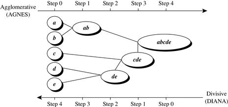
DIANA, the divisive method, proceeds in the contrasting way. All the objects are used to form one initial cluster. The cluster is split according to some principle such as the maximum Euclidean distance between the closest neighboring objects in the cluster. The cluster-splitting process repeats until, eventually, each new cluster contains only a single object.
A tree structure called a dendrogram is commonly used to represent the process of hierarchical clustering. It shows how objects are grouped together (in an agglomerative method) or partitioned (in a divisive method) step-by-step. Figure 10.7 shows a dendrogram for the five objects presented in Figure 10.6, where l = 0 shows the five objects as singleton clusters at level 0. At l = 1, objects a and b are grouped together to form the first cluster, and they stay together at all subsequent levels. We can also use a vertical axis to show the similarity scale between clusters. For example, when the similarity of two groups of objects, {a, b} and {c, d, e}, is roughly 0.16, they are merged together to form a single cluster.

A challenge with divisive methods is how to partition a large cluster into several smaller ones. For example, there are 2n − 1 − 1 possible ways to partition a set of n objects into two exclusive subsets, where n is the number of objects. When n is large, it is computationally prohibitive to examine all possibilities. Consequently, a divisive method typically uses heuristics in partitioning, which can lead to inaccurate results. For the sake of efficiency, divisive methods typically do not backtrack on partitioning decisions that have been made. Once a cluster is partitioned, any alternative partitioning of this cluster will not be considered again. Due to the challenges in divisive methods, there are many more agglomerative methods than divisive methods.
10.3.2 Distance Measures in Algorithmic Methods
Whether using an agglomerative method or a divisive method, a core need is to measure the distance between two clusters, where each cluster is generally a set of objects.
Four widely used measures for distance between clusters are as follows, where |p − p′| is the distance between two objects or points, p and p′; mi is the mean for cluster, Ci; and ni is the number of objects in Ci. They are also known as linkage measures.
![]() (10.3)
(10.3)
![]() (10.4)
(10.4)
![]() (10.5)
(10.5)
 (10.6)
When an algorithm uses the minimum distance, dmin(Ci, Cj), to measure the distance between clusters, it is sometimes called a nearest-neighbor clustering algorithm. Moreover, if the clustering process is terminated when the distance between nearest clusters exceeds a user-defined threshold, it is called a single-linkage algorithm. If we view the data points as nodes of a graph, with edges forming a path between the nodes in a cluster, then the merging of two clusters, Ci and Cj, corresponds to adding an edge between the nearest pair of nodes in Ci and Cj. Because edges linking clusters always go between distinct clusters, the resulting graph will generate a tree. Thus, an agglomerative hierarchical clustering algorithm that uses the minimum distance measure is also called a minimal spanning tree algorithm, where a spanning tree of a graph is a tree that connects all vertices, and a minimal spanning tree is the one with the least sum of edge weights.
When an algorithm uses the maximum distance, dmax(Ci, Cj), to measure the distance between clusters, it is sometimes called a farthest-neighbor clustering algorithm. If the clustering process is terminated when the maximum distance between nearest clusters exceeds a user-defined threshold, it is called a complete-linkage algorithm. By viewing data points as nodes of a graph, with edges linking nodes, we can think of each cluster as a complete subgraph, that is, with edges connecting all the nodes in the clusters. The distance between two clusters is determined by the most distant nodes in the two clusters. Farthest-neighbor algorithms tend to minimize the increase in diameter of the clusters at each iteration. If the true clusters are rather compact and approximately equal size, the method will produce high-quality clusters. Otherwise, the clusters produced can be meaningless.
The previous minimum and maximum measures represent two extremes in measuring the distance between clusters. They tend to be overly sensitive to outliers or noisy data. The use of mean or average distance is a compromise between the minimum and maximum distances and overcomes the outlier sensitivity problem. Whereas the mean distance is the simplest to compute, the average distance is advantageous in that it can handle categoric as well as numeric data. The computation of the mean vector for categoric data can be difficult or impossible to define.
Example 10.4
Single versus complete linkages
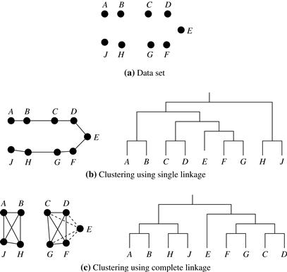
Let us apply hierarchical clustering to the data set of Figure 10.8(a). Figure 10.8(b) shows the dendrogram using single linkage. Figure 10.8(c) shows the case using complete linkage, where the edges between clusters {A, B, J, H} and {C, D, G, F, E} are omitted for ease of presentation. This example shows that by using single linkages we can find hierarchical clusters defined by local proximity, whereas complete linkage tends to find clusters opting for global closeness.
There are variations of the four essential linkage measures just discussed. For example, we can measure the distance between two clusters by the distance between the centroids (i.e., the central objects) of the clusters.
10.3.3 BIRCH: Multiphase Hierarchical Clustering Using Clustering Feature Trees
Balanced Iterative Reducing and Clustering using Hierarchies (BIRCH) is designed for clustering a large amount of numeric data by integrating hierarchical clustering (at the initial microclustering stage) and other clustering methods such as iterative partitioning (at the later macroclustering stage). It overcomes the two difficulties in agglomerative clustering methods: (1) scalability and (2) the inability to undo what was done in the previous step.
BIRCH uses the notions of clustering feature to summarize a cluster, and clustering feature tree (CF-tree) to represent a cluster hierarchy. These structures help the clustering method achieve good speed and scalability in large or even streaming databases, and also make it effective for incremental and dynamic clustering of incoming objects.
Consider a cluster of n d-dimensional data objects or points. The clustering feature (CF) of the cluster is a 3-D vector summarizing information about clusters of objects. It is defined as
![]() (10.7)
(10.7)
where LS is the linear sum of the n points (i.e., ![]() ), and SS is the square sum of the data points (i.e.,
), and SS is the square sum of the data points (i.e., ![]() ).
).
A clustering feature is essentially a summary of the statistics for the given cluster. Using a clustering feature, we can easily derive many useful statistics of a cluster. For example, the cluster’s centroid, x0, radius, R, and diameter, D, are
 (10.8)
 (10.9)
 (10.10)
Here, R is the average distance from member objects to the centroid, and D is the average pairwise distance within a cluster. Both R and D reflect the tightness of the cluster around the centroid.
Summarizing a cluster using the clustering feature can avoid storing the detailed information about individual objects or points. Instead, we only need a constant size of space to store the clustering feature. This is the key to BIRCH efficiency in space. Moreover, clustering features are additive. That is, for two disjoint clusters, C1 and C2, with the clustering features ![]() and
and ![]() , respectively, the clustering feature for the cluster that formed by merging C1 and C2 is simply
, respectively, the clustering feature for the cluster that formed by merging C1 and C2 is simply
![]() (10.11)
(10.11)
Example 10.5
Clustering feature
Suppose there are three points, (2, 5), (3, 2), and (4, 3), in a cluster, C1. The clustering feature of C1 is
![]()
Suppose that C1 is disjoint to a second cluster, C2, where ![]() . The clustering feature of a new cluster, C3, that is formed by merging C1 and C2, is derived by adding CF1 and CF2. That is,
. The clustering feature of a new cluster, C3, that is formed by merging C1 and C2, is derived by adding CF1 and CF2. That is,
![]()
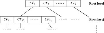
A CF-tree is a height-balanced tree that stores the clustering features for a hierarchical clustering. An example is shown in Figure 10.9. By definition, a nonleaf node in a tree has descendants or “children.” The nonleaf nodes store sums of the CFs of their children, and thus summarize clustering information about their children. A CF-tree has two parameters: branching factor, B, and threshold, T. The branching factor specifies the maximum number of children per nonleaf node. The threshold parameter specifies the maximum diameter of subclusters stored at the leaf nodes of the tree. These two parameters implicitly control the resulting tree’s size.
Given a limited amount of main memory, an important consideration in BIRCH is to minimize the time required for input/output (I/O). BIRCH applies a multiphase clustering technique: A single scan of the data set yields a basic, good clustering, and one or more additional scans can optionally be used to further improve the quality. The primary phases are
■ Phase 1: BIRCH scans the database to build an initial in-memory CF-tree, which can be viewed as a multilevel compression of the data that tries to preserve the data’s inherent clustering structure.
■ Phase 2: BIRCH applies a (selected) clustering algorithm to cluster the leaf nodes of the CF-tree, which removes sparse clusters as outliers and groups dense clusters into larger ones.
For Phase 1, the CF-tree is built dynamically as objects are inserted. Thus, the method is incremental. An object is inserted into the closest leaf entry (subcluster). If the diameter of the subcluster stored in the leaf node after insertion is larger than the threshold value, then the leaf node and possibly other nodes are split. After the insertion of the new object, information about the object is passed toward the root of the tree. The size of the CF-tree can be changed by modifying the threshold. If the size of the memory that is needed for storing the CF-tree is larger than the size of the main memory, then a larger threshold value can be specified and the CF-tree is rebuilt.
The rebuild process is performed by building a new tree from the leaf nodes of the old tree. Thus, the process of rebuilding the tree is done without the necessity of rereading all the objects or points. This is similar to the insertion and node split in the construction of B+-trees. Therefore, for building the tree, data has to be read just once. Some heuristics and methods have been introduced to deal with outliers and improve the quality of CF-trees by additional scans of the data. Once the CF-tree is built, any clustering algorithm, such as a typical partitioning algorithm, can be used with the CF-tree in Phase 2.
“How effective is BIRCH?” The time complexity of the algorithm is O(n), where n is the number of objects to be clustered. Experiments have shown the linear scalability of the algorithm with respect to the number of objects, and good quality of clustering of the data. However, since each node in a CF-tree can hold only a limited number of entries due to its size, a CF-tree node does not always correspond to what a user may consider a natural cluster. Moreover, if the clusters are not spherical in shape, BIRCH does not perform well because it uses the notion of radius or diameter to control the boundary of a cluster.
The ideas of clustering features and CF-trees have been applied beyond BIRCH. The ideas have been borrowed by many others to tackle problems of clustering streaming and dynamic data.
10.3.4 Chameleon: Multiphase Hierarchical Clustering Using Dynamic Modeling
Chameleon is a hierarchical clustering algorithm that uses dynamic modeling to determine the similarity between pairs of clusters. In Chameleon, cluster similarity is assessed based on (1) how well connected objects are within a cluster and (2) the proximity of clusters. That is, two clusters are merged if their interconnectivity is high and they are close together. Thus, Chameleon does not depend on a static, user-supplied model and can automatically adapt to the internal characteristics of the clusters being merged. The merge process facilitates the discovery of natural and homogeneous clusters and applies to all data types as long as a similarity function can be specified.
Figure 10.10 illustrates how Chameleon works. Chameleon uses a k-nearest-neighbor graph approach to construct a sparse graph, where each vertex of the graph represents a data object, and there exists an edge between two vertices (objects) if one object is among the k-most similar objects to the other. The edges are weighted to reflect the similarity between objects. Chameleon uses a graph partitioning algorithm to partition the k-nearest-neighbor graph into a large number of relatively small subclusters such that it minimizes the edge cut. That is, a cluster C is partitioned into subclusters Ci and Cj so as to minimize the weight of the edges that would be cut should C be bisected into Ci and Cj. It assesses the absolute interconnectivity between clusters Ci and Cj.
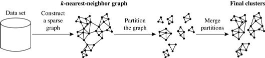
Figure 10.10 Chameleon: hierarchical clustering based on k-nearest neighbors and dynamic modeling. Source: Based on Karypis, Han, and Kumar [KHK99].
Chameleon then uses an agglomerative hierarchical clustering algorithm that iteratively merges subclusters based on their similarity. To determine the pairs of most similar subclusters, it takes into account both the interconnectivity and the closeness of the clusters. Specifically, Chameleon determines the similarity between each pair of clusters Ci and Cj according to their relative interconnectivity, RI(Ci, Cj), and their relative closeness, RC(Ci, Cj).
■ The relative interconnectivity, RI(Ci, Cj), between two clusters, Ci and Cj, is defined as the absolute interconnectivity between Ci and Cj, normalized with respect to the internal interconnectivity of the two clusters, Ci and Cj. That is,
![]() (10.12)
(10.12)
where EC{Ci, Cj} is the edge cut as previously defined for a cluster containing both Ci and Cj. Similarly, ECCi (or ECCj) is the minimum sum of the cut edges that partition Ci (or Cj) into two roughly equal parts.
■ The relative closeness, RC(Ci, Cj), between a pair of clusters, Ci and Cj, is the absolute closeness between Ci and Cj, normalized with respect to the internal closeness of the two clusters, Ci and Cj. It is defined as
 (10.13)
where ![]() is the average weight of the edges that connect vertices in Ci to vertices in Cj, and
is the average weight of the edges that connect vertices in Ci to vertices in Cj, and ![]() (or
(or ![]() ) is the average weight of the edges that belong to the min-cut bisector of cluster Ci(or Cj).
) is the average weight of the edges that belong to the min-cut bisector of cluster Ci(or Cj).
Chameleon has been shown to have greater power at discovering arbitrarily shaped clusters of high quality than several well-known algorithms such as BIRCH and density-based DBSCAN (Section 10.4.1). However, the processing cost for high-dimensional data may require O(n2) time for n objects in the worst case.
10.3.5 Probabilistic Hierarchical Clustering
Algorithmic hierarchical clustering methods using linkage measures tend to be easy to understand and are often efficient in clustering. They are commonly used in many clustering analysis applications. However, algorithmic hierarchical clustering methods can suffer from several drawbacks. First, choosing a good distance measure for hierarchical clustering is often far from trivial. Second, to apply an algorithmic method, the data objects cannot have any missing attribute values. In the case of data that are partially observed (i.e., some attribute values of some objects are missing), it is not easy to apply an algorithmic hierarchical clustering method because the distance computation cannot be conducted. Third, most of the algorithmic hierarchical clustering methods are heuristic, and at each step locally search for a good merging/splitting decision. Consequently, the optimization goal of the resulting cluster hierarchy can be unclear.
Probabilistic hierarchical clustering aims to overcome some of these disadvantages by using probabilistic models to measure distances between clusters.
One way to look at the clustering problem is to regard the set of data objects to be clustered as a sample of the underlying data generation mechanism to be analyzed or, formally, the generative model. For example, when we conduct clustering analysis on a set of marketing surveys, we assume that the surveys collected are a sample of the opinions of all possible customers. Here, the data generation mechanism is a probability distribution of opinions with respect to different customers, which cannot be obtained directly and completely. The task of clustering is to estimate the generative model as accurately as possible using the observed data objects to be clustered.
In practice, we can assume that the data generative models adopt common distribution functions, such as Gaussian distribution or Bernoulli distribution, which are governed by parameters. The task of learning a generative model is then reduced to finding the parameter values for which the model best fits the observed data set.
Example 10.6
Generative model
Suppose we are given a set of 1-D points X = {x1, …, xn} for clustering analysis. Let us assume that the data points are generated by a Gaussian distribution,
 (10.14)
where the parameters are μ (the mean) and σ2 (the variance).
The probability that a point xi ∈ X is then generated by the model is
![]() (10.15)
(10.15)
Consequently, the likelihood that X is generated by the model is
 (10.16)
The task of learning the generative model is to find the parameters μ and σ2 such that the likelihood ![]() is maximized, that is, finding
is maximized, that is, finding
![]() (10.17)
(10.17)
where ![]() is called the maximum likelihood.
is called the maximum likelihood.
Given a set of objects, the quality of a cluster formed by all the objects can be measured by the maximum likelihood. For a set of objects partitioned into m clusters C1, …, Cm, the quality can be measured by
 (10.18)
where P() is the maximum likelihood. If we merge two clusters, Cj1 and Cj2, into a cluster, Cj1 ∪ Cj2, then, the change in quality of the overall clustering is
 (10.19)
When choosing to merge two clusters in hierarchical clustering, ![]() is constant for any pair of clusters. Therefore, given clusters C1 and C2, the distance between them can be measured by
is constant for any pair of clusters. Therefore, given clusters C1 and C2, the distance between them can be measured by
![]() (10.20)
(10.20)
A probabilistic hierarchical clustering method can adopt the agglomerative clustering framework, but use probabilistic models (Eq. 10.20) to measure the distance between clusters.
Upon close observation of Eq. (10.19), we see that merging two clusters may not always lead to an improvement in clustering quality, that is, ![]() may be less than 1. For example, assume that Gaussian distribution functions are used in the model of Figure 10.11. Although merging clusters C1 and C2 results in a cluster that better fits a Gaussian distribution, merging clusters C3 and C4 lowers the clustering quality because no Gaussian functions can fit the merged cluster well.
may be less than 1. For example, assume that Gaussian distribution functions are used in the model of Figure 10.11. Although merging clusters C1 and C2 results in a cluster that better fits a Gaussian distribution, merging clusters C3 and C4 lowers the clustering quality because no Gaussian functions can fit the merged cluster well.
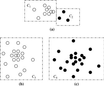
Figure 10.11 Merging clusters in probabilistic hierarchical clustering: (a) Merging clusters C1 and C2 leads to an increase in overall cluster quality, but merging clusters (b) C3 and (c) C4 does not.
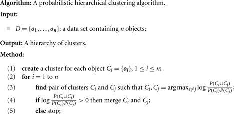
Based on this observation, a probabilistic hierarchical clustering scheme can start with one cluster per object, and merge two clusters, Ci and Cj, if the distance between them is negative. In each iteration, we try to find Ci and Cj so as to maximize ![]() . The iteration continues as long as
. The iteration continues as long as ![]() , that is, as long as there is an improvement in clustering quality. The pseudocode is given in Figure 10.12.
, that is, as long as there is an improvement in clustering quality. The pseudocode is given in Figure 10.12.
Probabilistic hierarchical clustering methods are easy to understand, and generally have the same efficiency as algorithmic agglomerative hierarchical clustering methods; in fact, they share the same framework. Probabilistic models are more interpretable, but sometimes less flexible than distance metrics. Probabilistic models can handle partially observed data. For example, given a multidimensional data set where some objects have missing values on some dimensions, we can learn a Gaussian model on each dimension independently using the observed values on the dimension. The resulting cluster hierarchy accomplishes the optimization goal of fitting data to the selected probabilistic models.
A drawback of using probabilistic hierarchical clustering is that it outputs only one hierarchy with respect to a chosen probabilistic model. It cannot handle the uncertainty of cluster hierarchies. Given a data set, there may exist multiple hierarchies that fit the observed data. Neither algorithmic approaches nor probabilistic approaches can find the distribution of such hierarchies. Recently, Bayesian tree-structured models have been developed to handle such problems. Bayesian and other sophisticated probabilistic clustering methods are considered advanced topics and are not covered in this book.