
5.2 Data Cube Computation Methods
Data cube computation is an essential task in data warehouse implementation. The precomputation of all or part of a data cube can greatly reduce the response time and enhance the performance of online analytical processing. However, such computation is challenging because it may require substantial computational time and storage space. This section explores efficient methods for data cube computation. Section 5.2.1 describes the multiway array aggregation (MultiWay) method for computing full cubes. Section 5.2.2 describes a method known as BUC, which computes iceberg cubes from the apex cuboid downward. Section 5.2.3 describes the Star-Cubing method, which integrates top-down and bottom-up computation.
Finally, Section 5.2.4 describes a shell-fragment cubing approach that computes shell fragments for efficient high-dimensional OLAP. To simplify our discussion, we exclude the cuboids that would be generated by climbing up any existing hierarchies for the dimensions. Those cube types can be computed by extension of the discussed methods. Methods for the efficient computation of closed cubes are left as an exercise for interested readers.
5.2.1 Multiway Array Aggregation for Full Cube Computation
The multiway array aggregation (or simply MultiWay) method computes a full data cube by using a multidimensional array as its basic data structure. It is a typical MOLAP approach that uses direct array addressing, where dimension values are accessed via the position or index of their corresponding array locations. Hence, MultiWay cannot perform any value-based reordering as an optimization technique. A different approach is developed for the array-based cube construction, as follows:
1. Partition the array into chunks. A chunk is a subcube that is small enough to fit into the memory available for cube computation. Chunking is a method for dividing an n-dimensional array into small n-dimensional chunks, where each chunk is stored as an object on disk. The chunks are compressed so as to remove wasted space resulting from empty array cells. A cell is empty if it does not contain any valid data (i.e., its cell count is 0). For instance, “chunkID + offset” can be used as a cell-addressing mechanism to compress a sparse array structure and when searching for cells within a chunk. Such a compression technique is powerful at handling sparse cubes, both on disk and in memory.
2. Compute aggregates by visiting (i.e., accessing the values at) cube cells. The order in which cells are visited can be optimized so as to minimize the number of times that each cell must be revisited, thereby reducing memory access and storage costs. The trick is to exploit this ordering so that portions of the aggregate cells in multiple cuboids can be computed simultaneously, and any unnecessary revisiting of cells is avoided.
This chunking technique involves “overlapping” some of the aggregation computations; therefore, it is referred to as multiway array aggregation. It performs simultaneous aggregation, that is, it computes aggregations simultaneously on multiple dimensions.
We explain this approach to array-based cube construction by looking at a concrete example.
Example 5.4
Multiway array cube computation
Consider a 3-D data array containing the three dimensions A, B, and C. The 3-D array is partitioned into small, memory-based chunks. In this example, the array is partitioned into 64 chunks as shown in Figure 5.3. Dimension A is organized into four equal-sized partitions: a0, a1, a2, and a3. Dimensions B and C are similarly organized into four partitions each. Chunks 1, 2, …, 64 correspond to the subcubes a0b0c0, a1b0c0, …, a3b3c3, respectively. Suppose that the cardinality of the dimensions A, B, and C is 40, 400, and 4000, respectively. Thus, the size of the array for each dimension, A, B, and C, is also 40, 400, and 4000, respectively. The size of each partition in A, B, and C is therefore 10, 100, and 1000, respectively. Full materialization of the corresponding data cube involves the computation of all the cuboids defining this cube. The resulting full cube consists of the following cuboids:
■ The base cuboid, denoted by ABC (from which all the other cuboids are directly or indirectly computed). This cube is already computed and corresponds to the given 3-D array.
■ The 2-D cuboids, AB, AC, and BC, which respectively correspond to the group-by’s AB, AC, and BC. These cuboids must be computed.
■ The 1-D cuboids, A, B, and C, which respectively correspond to the group-by’s A, B, and C. These cuboids must be computed.
■ The 0-D (apex) cuboid, denoted by all, which corresponds to the group-by (); that is, there is no group-by here. This cuboid must be computed. It consists of only one value. If, say, the data cube measure is count, then the value to be computed is simply the total count of all the tuples in ABC.
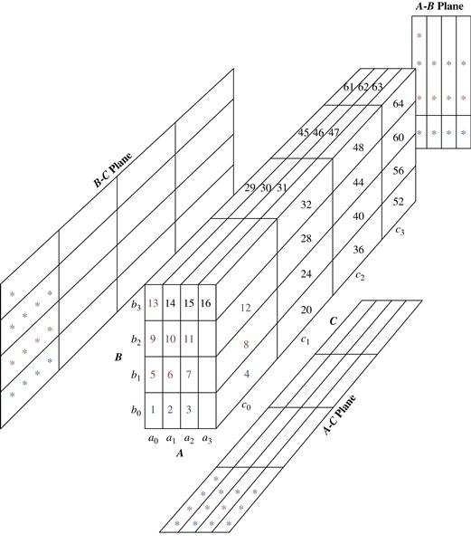
Figure 5.3 A 3-D array for the dimensions A, B, and C, organized into 64 chunks. Each chunk is small enough to fit into the memory available for cube computation. The ∗’s indicate the chunks from 1 to 13 that have been aggregated so far in the process.
Let’s look at how the multiway array aggregation technique is used in this computation. There are many possible orderings with which chunks can be read into memory for use in cube computation. Consider the ordering labeled from 1 to 64, shown in Figure 5.3. Suppose we want to compute the b0c0 chunk of the BC cuboid. We allocate space for this chunk in chunk memory. By scanning ABC chunks 1 through 4, the b0c0 chunk is computed. That is, the cells for b0c0 are aggregated over a0 to a3. The chunk memory can then be assigned to the next chunk, b1c0, which completes its aggregation after the scanning of the next four ABC chunks: 5 through 8. Continuing in this way, the entire BC cuboid can be computed. Therefore, only one BC chunk needs to be in memory at a time, for the computation of all the BC chunks.
In computing the BC cuboid, we will have scanned each of the 64 chunks. “Is there a way to avoid having to rescan all of these chunks for the computation of other cuboids such as AC and AB?” The answer is, most definitely, yes. This is where the “multiway computation” or “simultaneous aggregation” idea comes in. For example, when chunk 1 (i.e., a0b0c0) is being scanned (say, for the computation of the 2-D chunk b0c0 of BC, as described previously), all of the other 2-D chunks relating to a0b0c0 can be simultaneously computed. That is, when a0b0c0 is being scanned, each of the three chunks (b0c0, a0c0, and a0b0) on the three 2-D aggregation planes (BC, AC, and AB) should be computed then as well. In other words, multiway computation simultaneously aggregates to each of the 2-D planes while a 3-D chunk is in memory.
Now let’s look at how different orderings of chunk scanning and of cuboid computation can affect the overall data cube computation efficiency. Recall that the size of the dimensions A, B, and C is 40, 400, and 4000, respectively. Therefore, the largest 2-D plane is BC (of size 400 × 4000 = 1,600,000). The second largest 2-D plane is AC (of size 40 × 4000 = 160,000). AB is the smallest 2-D plane (of size 40 × 400 = 16,000).
Suppose that the chunks are scanned in the order shown, from chunks 1 to 64. As previously mentioned, b0c0 is fully aggregated after scanning the row containing chunks 1 through 4; b1c0 is fully aggregated after scanning chunks 5 through 8, and so on. Thus, we need to scan four chunks of the 3-D array to fully compute one chunk of the BC cuboid (where BC is the largest of the 2-D planes). In other words, by scanning in this order, one BC chunk is fully computed for each row scanned. In comparison, the complete computation of one chunk of the second largest 2-D plane, AC, requires scanning 13 chunks, given the ordering from 1 to 64. That is, a0c0 is fully aggregated only after the scanning of chunks 1, 5, 9, and 13.
Finally, the complete computation of one chunk of the smallest 2-D plane, AB, requires scanning 49 chunks. For example, a0b0 is fully aggregated after scanning chunks 1, 17, 33, and 49. Hence, AB requires the longest scan of chunks to complete its computation. To avoid bringing a 3-D chunk into memory more than once, the minimum memory requirement for holding all relevant 2-D planes in chunk memory, according to the chunk ordering of 1 to 64, is as follows: 40 × 400 (for the whole AB plane) + 40 × 1000 (for one column of the AC plane) + 100 × 1000 (for one BC plane chunk) = 16,000 + 40,000 + 100,000 = 156,000 memory units.
Suppose, instead, that the chunks are scanned in the order 1, 17, 33, 49, 5, 21, 37, 53, and so on. That is, suppose the scan is in the order of first aggregating toward the AB plane, and then toward the AC plane, and lastly toward the BC plane. The minimum memory requirement for holding 2-D planes in chunk memory would be as follows: 400 × 4000 (for the whole BC plane) + 10 × 4000 (for one AC plane row) + 10 × 100 (for one AB plane chunk) = 1,600,000 + 40,000 + 1000 = 1,641,000 memory units. Notice that this is more than 10 times the memory requirement of the scan ordering of 1 to 64.
Similarly, we can work out the minimum memory requirements for the multiway computation of the 1-D and 0-D cuboids. Figure 5.4 shows the most efficient way to compute 1-D cuboids. Chunks for 1-D cuboids A and B are computed during the computation of the smallest 2-D cuboid, AB. The smallest 1-D cuboid, A, will have all of its chunks allocated in memory, whereas the larger 1-D cuboid, B, will have only one chunk allocated in memory at a time. Similarly, chunk C is computed during the computation of the second smallest 2-D cuboid, AC, requiring only one chunk in memory at a time. Based on this analysis, we see that the most efficient ordering in this array cube computation is the chunk ordering of 1 to 64, with the stated memory allocation strategy.
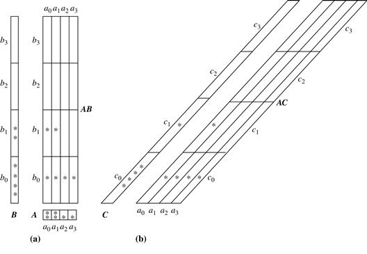
Figure 5.4 Memory allocation and computation order for computing Example 5.4’s 1-D cuboids. (a) The 1-D cuboids, A and B, are aggregated during the computation of the smallest 2-D cuboid, AB. (b) The 1-D cuboid, C, is aggregated during the computation of the second smallest 2-D cuboid, AC. The ∗’s represent chunks that, so far, have been aggregated to.
Example 5.4 assumes that there is enough memory space for one-pass cube computation (i.e., to compute all of the cuboids from one scan of all the chunks). If there is insufficient memory space, the computation will require more than one pass through the 3-D array. In such cases, however, the basic principle of ordered chunk computation remains the same. MultiWay is most effective when the product of the cardinalities of dimensions is moderate and the data are not too sparse. When the dimensionality is high or the data are very sparse, the in-memory arrays become too large to fit in memory, and this method becomes infeasible.
With the use of appropriate sparse array compression techniques and careful ordering of the computation of cuboids, it has been shown by experiments that MultiWay array cube computation is significantly faster than traditional ROLAP (relational record-based) computation. Unlike ROLAP, the array structure of MultiWay does not require saving space to store search keys. Furthermore, MultiWay uses direct array addressing, which is faster than ROLAP’s key-based addressing search strategy. For ROLAP cube computation, instead of cubing a table directly, it can be faster to convert the table to an array, cube the array, and then convert the result back to a table. However, this observation works only for cubes with a relatively small number of dimensions, because the number of cuboids to be computed is exponential to the number of dimensions.
“What would happen if we tried to use MultiWay to compute iceberg cubes?” Remember that the Apriori property states that if a given cell does not satisfy minimum support, then neither will any of its descendants. Unfortunately, MultiWay’s computation starts from the base cuboid and progresses upward toward more generalized, ancestor cuboids. It cannot take advantage of Apriori pruning, which requires a parent node to be computed before its child (i.e., more specific) nodes. For example, if the count of a cell c in, say, AB, does not satisfy the minimum support specified in the iceberg condition, we cannot prune away cell c, because the count of c’s ancestors in the A or B cuboids may be greater than the minimum support, and their computation will need aggregation involving the count of c.
5.2.2 BUC: Computing Iceberg Cubes from the Apex Cuboid Downward
BUC is an algorithm for the computation of sparse and iceberg cubes. Unlike MultiWay, BUC constructs the cube from the apex cuboid toward the base cuboid. This allows BUC to share data partitioning costs. This processing order also allows BUC to prune during construction, using the Apriori property.
Figure 5.5 shows a lattice of cuboids, making up a 3-D data cube with the dimensions A, B, and C. The apex (0-D) cuboid, representing the concept all (i.e., (∗, ∗, ∗)), is at the top of the lattice. This is the most aggregated or generalized level. The 3-D base cuboid, ABC, is at the bottom of the lattice. It is the least aggregated (most detailed or specialized) level. This representation of a lattice of cuboids, with the apex at the top and the base at the bottom, is commonly accepted in data warehousing. It consolidates the notions of drill-down (where we can move from a highly aggregated cell to lower, more detailed cells) and roll-up (where we can move from detailed, low-level cells to higher-level, more aggregated cells).
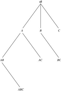
Figure 5.5 BUC’s exploration for a 3-D data cube computation. Note that the computation starts from the apex cuboid.
BUC stands for “Bottom-Up Construction.” However, according to the lattice convention described before and used throughout this book, the BUC processing order is actually top-down! The BUC authors view a lattice of cuboids in the reverse order, with the apex cuboid at the bottom and the base cuboid at the top. In that view, BUC does bottom-up construction. However, because we adopt the application worldview where drill-down refers to drilling from the apex cuboid down toward the base cuboid, the exploration process of BUC is regarded as top-down. BUC’s exploration for the computation of a 3-D data cube is shown in Figure 5.5.
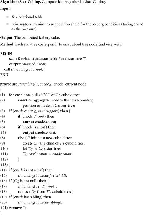
The BUC algorithm is shown on the next page in Figure 5.6. We first give an explanation of the algorithm and then follow up with an example. Initially, the algorithm is called with the input relation (set of tuples). BUC aggregates the entire input (line 1) and writes the resulting total (line 3). (Line 2 is an optimization feature that is discussed later in our example.) For each dimension d (line 4), the input is partitioned on d (line 6). On return from Partition(), dataCount contains the total number of tuples for each distinct value of dimension d. Each distinct value of d forms its own partition. Line 8 iterates through each partition. Line 10 tests the partition for minimum support. That is, if the number of tuples in the partition satisfies (i.e., is ≥) the minimum support, then the partition becomes the input relation for a recursive call made to BUC, which computes the iceberg cube on the partitions for dimensions d + 1 to numDims (line 12).
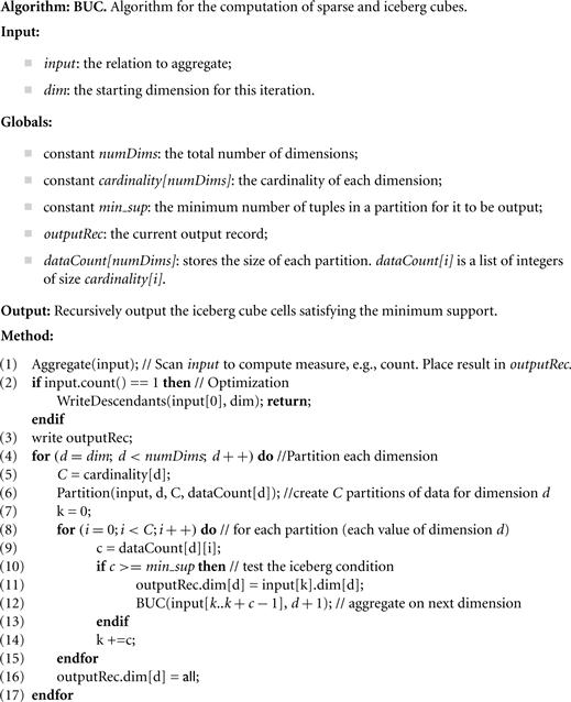
Figure 5.6 BUC algorithm for sparse or iceberg cube computation. Source: Beyer and Ramakrishnan [BR99].
Note that for a full cube (i.e., where minimum support in the having clause is 1), the minimum support condition is always satisfied. Thus, the recursive call descends one level deeper into the lattice. On return from the recursive call, we continue with the next partition for d. After all the partitions have been processed, the entire process is repeated for each of the remaining dimensions.
Example 5.5
BUC construction of an iceberg cube
Consider the iceberg cube expressed in SQL as follows:
compute cube iceberg_cube as
select A, B, C, D, count(*)
from R
cube by A, B, C, D
having count(*) > = 3
Let’s see how BUC constructs the iceberg cube for the dimensions A, B, C, and D, where 3 is the minimum support count. Suppose that dimension A has four distinct values, a1, a2, a3, a4; B has four distinct values, b1, b2, b3, b4; C has two distinct values, c1, c2; and D has two distinct values, d1, d2. If we consider each group-by to be a partition, then we must compute every combination of the grouping attributes that satisfy the minimum support (i.e., that have three tuples).
Figure 5.7 illustrates how the input is partitioned first according to the different attribute values of dimension A, and then B, C, and D. To do so, BUC scans the input, aggregating the tuples to obtain a count for all, corresponding to the cell (∗, ∗, ∗, ∗). Dimension A is used to split the input into four partitions, one for each distinct value of A. The number of tuples (counts) for each distinct value of A is recorded in dataCount.
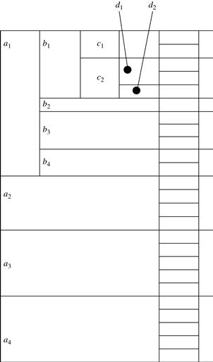
BUC uses the Apriori property to save time while searching for tuples that satisfy the iceberg condition. Starting with A dimension value, a1, the a1 partition is aggregated, creating one tuple for the A group-by, corresponding to the cell (a1, ∗, ∗, ∗). Suppose (a1, ∗, ∗, ∗) satisfies the minimum support, in which case a recursive call is made on the partition for a1. BUC partitions a1 on the dimension B. It checks the count of (a1, b1, ∗, ∗) to see if it satisfies the minimum support. If it does, it outputs the aggregated tuple to the AB group-by and recurses on (a1, b1, ∗, ∗) to partition on C, starting with c1. Suppose the cell count for (a1, b1, c1, ∗) is 2, which does not satisfy the minimum support. According to the Apriori property, if a cell does not satisfy the minimum support, then neither can any of its descendants. Therefore, BUC prunes any further exploration of (a1, b1, c1, ∗). That is, it avoids partitioning this cell on dimension D. It backtracks to the a1, b1 partition and recurses on (a1, b1, c2, ∗), and so on. By checking the iceberg condition each time before performing a recursive call, BUC saves a great deal of processing time whenever a cell’s count does not satisfy the minimum support.
The partition process is facilitated by a linear sorting method, CountingSort. CountingSort is fast because it does not perform any key comparisons to find partition boundaries. In addition, the counts computed during the sort can be reused to compute the group-by’s in BUC. Line 2 is an optimization for partitions having a count of 1 such as (a1, b2, ∗, ∗) in our example. To save on partitioning costs, the count is written to each of the tuple’s descendant group-by’s. This is particularly useful since, in practice, many partitions have a single tuple.
The BUC performance is sensitive to the order of the dimensions and to skew in the data. Ideally, the most discriminating dimensions should be processed first. Dimensions should be processed in the order of decreasing cardinality. The higher the cardinality, the smaller the partitions, and thus the more partitions there will be, thereby providing BUC with a greater opportunity for pruning. Similarly, the more uniform a dimension (i.e., having less skew), the better it is for pruning.
BUC’s major contribution is the idea of sharing partitioning costs. However, unlike MultiWay, it does not share the computation of aggregates between parent and child group-by’s. For example, the computation of cuboid AB does not help that of ABC. The latter needs to be computed essentially from scratch.
5.2.3 Star-Cubing: Computing Iceberg Cubes Using a Dynamic Star-Tree Structure
In this section, we describe the Star-Cubing algorithm for computing iceberg cubes. Star-Cubing combines the strengths of the other methods we have studied up to this point. It integrates top-down and bottom-up cube computation and explores both multidimensional aggregation (similar to MultiWay) and Apriori-like pruning (similar to BUC). It operates from a data structure called a star-tree, which performs lossless data compression, thereby reducing the computation time and memory requirements.
The Star-Cubing algorithm explores both the bottom-up and top-down computation models as follows: On the global computation order, it uses the bottom-up model. However, it has a sublayer underneath based on the top-down model, which explores the notion of shared dimensions, as we shall see in the following. This integration allows the algorithm to aggregate on multiple dimensions while still partitioning parent group-by’s and pruning child group-by’s that do not satisfy the iceberg condition.
Star-Cubing’s approach is illustrated in Figure 5.8 for a 4-D data cube computation. If we were to follow only the bottom-up model (similar to MultiWay), then the cuboids marked as pruned by Star-Cubing would still be explored. Star-Cubing is able to prune the indicated cuboids because it considers shared dimensions. ACD/A means cuboid ACD has shared dimension A, ABD/AB means cuboid ABD has shared dimension AB, ABC/ABC means cuboid ABC has shared dimension ABC, and so on. This comes from the generalization that all the cuboids in the subtree rooted at ACD include dimension A, all those rooted at ABD include dimensions AB, and all those rooted at ABC include dimensions ABC (even though there is only one such cuboid). We call these common dimensions the shared dimensions of those particular subtrees.
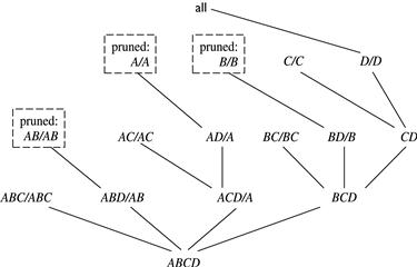
The introduction of shared dimensions facilitates shared computation. Because the shared dimensions are identified early on in the tree expansion, we can avoid recomputing them later. For example, cuboid AB extending from ABD in Figure 5.8 would actually be pruned because AB was already computed in ABD/AB. Similarly, cuboid A extending from AD would also be pruned because it was already computed in ACD/A.
Shared dimensions allow us to do Apriori-like pruning if the measure of an iceberg cube, such as count, is antimonotonic. That is, if the aggregate value on a shared dimension does not satisfy the iceberg condition, then all the cells descending from this shared dimension cannot satisfy the iceberg condition either. These cells and their descendants can be pruned because these descendant cells are, by definition, more specialized (i.e., contain more dimensions) than those in the shared dimension(s). The number of tuples covered by the descendant cells will be less than or equal to the number of tuples covered by the shared dimensions. Therefore, if the aggregate value on a shared dimension fails the iceberg condition, the descendant cells cannot satisfy it either.
To explain how the Star-Cubing algorithm works, we need to explain a few more concepts, namely, cuboid trees, star-nodes, and star-trees.
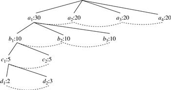
We use trees to represent individual cuboids. Figure 5.9 shows a fragment of the cuboid tree of the base cuboid, ABCD. Each level in the tree represents a dimension, and each node represents an attribute value. Each node has four fields: the attribute value, aggregate value, pointer to possible first child, and pointer to possible first sibling. Tuples in the cuboid are inserted one by one into the tree. A path from the root to a leaf node represents a tuple. For example, node c2 in the tree has an aggregate (count) value of 5, which indicated that there are five tuples of value (a1, b1, c2, ∗). This representation collapses the common prefixes to save memory usage and allows us to aggregate the values at internal nodes. With aggregate values at internal nodes, we can prune based on shared dimensions. For example, the AB cuboid tree can be used to prune possible cells in ABD.
If the single-dimensional aggregate on an attribute value p does not satisfy the iceberg condition, it is useless to distinguish such nodes in the iceberg cube computation. Thus, the node p can be replaced by ∗ so that the cuboid tree can be further compressed. We say that the node p in an attribute A is a star-node if the single-dimensional aggregate on p does not satisfy the iceberg condition; otherwise, p is a non-star-node. A cuboid tree that is compressed using star-nodes is called a star-tree.
Example 5.7
Star-tree construction
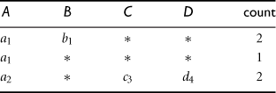
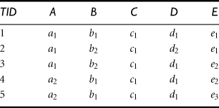
A base cuboid table is shown in Table 5.1. There are five tuples and four dimensions. The cardinalities for dimensions A, B, C, D are 2, 4, 4, 4, respectively. The one-dimensional aggregates for all attributes are shown in Table 5.2. Suppose min_sup = 2 in the iceberg condition. Clearly, only attribute values a1, a2, b1, c3, d4 satisfy the condition. All other values are below the threshold and thus become star-nodes. By collapsing star-nodes, the reduced base table is Table 5.3. Notice that the table contains two fewer rows and also fewer distinct values than Table 5.1.
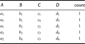
Table 5.2
| Dimension | count = 1 | count ≥ 2 |
| A | — | a1(3), a2(2) |
| B | b2, b3, b4 | b1(2) |
| C | c1, c2, c4 | c3(2) |
| D | d1, d2, d3 | d4(2) |
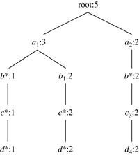
We use the reduced base table to construct the cuboid tree because it is smaller. The resultant star-tree is shown in Figure 5.10.
Now, let’s see how the Star-Cubing algorithm uses star-trees to compute an iceberg cube. The algorithm is given later in Figure 5.13.
Example 5.8
Star-Cubing
Using the star-tree generated in Example 5.7 (Figure 5.10), we start the aggregation process by traversing in a bottom-up fashion. Traversal is depth-first. The first stage (i.e., the processing of the first branch of the tree) is shown in Figure 5.11. The leftmost tree in the figure is the base star-tree. Each attribute value is shown with its corresponding aggregate value. In addition, subscripts by the nodes in the tree show the traversal order. The remaining four trees are BCD, ACD/A, ABD/AB, and ABC/ABC. They are the child trees of the base star-tree, and correspond to the level of 3-D cuboids above the base cuboid in Figure 5.8. The subscripts in them correspond to the same subscripts in the base tree—they denote the step or order in which they are created during the tree traversal. For example, when the algorithm is at step 1, the BCD child tree root is created. At step 2, the ACD/A child tree root is created. At step 3, the ABD/AB tree root and the b∗ node in BCD are created.
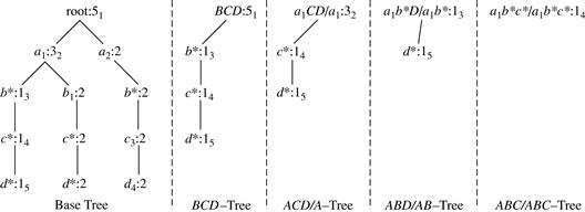
When the algorithm has reached step 5, the trees in memory are exactly as shown in Figure 5.11. Because depth-first traversal has reached a leaf at this point, it starts backtracking. Before traversing back, the algorithm notices that all possible nodes in the base dimension (ABC) have been visited. This means the ABC/ABC tree is complete, so the count is output and the tree is destroyed. Similarly, upon moving back from d∗ to c∗ and seeing that c∗ has no siblings, the count in ABD/AB is also output and the tree is destroyed.
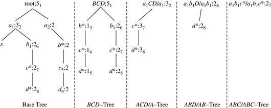
When the algorithm is at b∗ during the backtraversal, it notices that there exists a sibling in b1. Therefore, it will keep ACD/A in memory and perform a depth-first search on b1 just as it did on b∗. This traversal and the resultant trees are shown in Figure 5.12. The child trees ABD/AB and ABC/ABC are created again but now with the new values from the b1 subtree. For example, notice that the aggregate count of c∗ in the ACD/A tree has increased from 1 to 3. The trees that remained intact during the last traversal are reused and the new aggregate values are added on. For instance, another branch is added to the BCD tree.
Just like before, the algorithm will reach a leaf node at d∗ and traverse back. This time, it will reach a1 and notice that there exists a sibling in a2. In this case, all child trees except BCD in Figure 5.12 are destroyed. Afterward, the algorithm will perform the same traversal on a2. BCD continues to grow while the other subtrees start fresh with a2 instead of a1.
A node must satisfy two conditions in order to generate child trees: (1) the measure of the node must satisfy the iceberg condition; and (2) the tree to be generated must include at least one non-star-node (i.e., nontrivial). This is because if all the nodes were star-nodes, then none of them would satisfy min_sup. Therefore, it would be a complete waste to compute them. This pruning is observed in Figures 5.11 and 5.12. For example, the left subtree extending from node a1 in the base tree in Figure 5.11 does not include any nonstar-nodes. Therefore, the a1CD/a1 subtree should not have been generated. It is shown, however, for illustration of the child tree generation process.
Star-Cubing is sensitive to the ordering of dimensions, as with other iceberg cube construction algorithms. For best performance, the dimensions are processed in order of decreasing cardinality. This leads to a better chance of early pruning, because the higher the cardinality, the smaller the partitions, and therefore the higher possibility that the partition will be pruned.
Star-Cubing can also be used for full cube computation. When computing the full cube for a dense data set, Star-Cubing’s performance is comparable with MultiWay and is much faster than BUC. If the data set is sparse, Star-Cubing is significantly faster than MultiWay and faster than BUC, in most cases. For iceberg cube computation, Star-Cubing is faster than BUC, where the data are skewed and the speed-up factor increases as min_sup decreases.
5.2.4 Precomputing Shell Fragments for Fast High-Dimensional OLAP
Recall the reason that we are interested in precomputing data cubes: Data cubes facilitate fast OLAP in a multidimensional data space. However, a full data cube of high dimensionality needs massive storage space and unrealistic computation time. Iceberg cubes provide a more feasible alternative, as we have seen, wherein the iceberg condition is used to specify the computation of only a subset of the full cube’s cells. However, although an iceberg cube is smaller and requires less computation time than its corresponding full cube, it is not an ultimate solution.
For one, the computation and storage of the iceberg cube can still be costly. For example, if the base cuboid cell, (a1, a2, …, a60), passes minimum support (or the iceberg threshold), it will generate 260 iceberg cube cells. Second, it is difficult to determine an appropriate iceberg threshold. Setting the threshold too low will result in a huge cube, whereas setting the threshold too high may invalidate many useful applications. Third, an iceberg cube cannot be incrementally updated. Once an aggregate cell falls below the iceberg threshold and is pruned, its measure value is lost. Any incremental update would require recomputing the cells from scratch. This is extremely undesirable for large real-life applications where incremental appending of new data is the norm.
One possible solution, which has been implemented in some commercial data warehouse systems, is to compute a thin cube shell. For example, we could compute all cuboids with three dimensions or less in a 60-dimensional data cube, resulting in a cube shell of size 3. The resulting cuboids set would require much less computation and storage than the full 60-dimensional data cube. However, there are two disadvantages to this approach. First, we would still need to compute  cuboids, each with many cells. Second, such a cube shell does not support high-dimensional OLAP because (1) it does not support OLAP on four or more dimensions, and (2) it cannot even support drilling along three dimensions, such as, say, (A4, A5, A6), on a subset of data selected based on the constants provided in three other dimensions, such as (A1, A2, A3), because this essentially requires the computation of the corresponding 6-D cuboid. (Notice that there is no cell in cuboid (A4, A5, A6) computed for any particular constant set, such as (a1, a2, a3), associated with dimensions (A1, A2, A3).)
Instead of computing a cube shell, we can compute only portions or fragments of it. This section discusses the shell fragment approach for OLAP query processing. It is based on the following key observation about OLAP in high-dimensional space. Although a data cube may contain many dimensions, most OLAP operations are performed on only a small number of dimensions at a time. In other words, an OLAP query is likely to ignore many dimensions (i.e., treating them as irrelevant), fix some dimensions (e.g., using query constants as instantiations), and leave only a few to be manipulated (for drilling, pivoting, etc.). This is because it is neither realistic nor fruitful for anyone to comprehend the changes of thousands of cells involving tens of dimensions simultaneously in a high-dimensional space at the same time.
Instead, it is more natural to first locate some cuboids of interest and then drill along one or two dimensions to examine the changes of a few related dimensions. Most analysts will only need to examine, at any one moment, the combinations of a small number of dimensions. This implies that if multidimensional aggregates can be computed quickly on a small number of dimensions inside a high-dimensional space, we may still achieve fast OLAP without materializing the original high-dimensional data cube. Computing the full cube (or, often, even an iceberg cube or cube shell) can be excessive. Instead, a semi-online computation model with certain preprocessing may offer a more feasible solution. Given a base cuboid, some quick preparation computation can be done first (i.e., offline). After that, a query can then be computed online using the preprocessed data.
The shell fragment approach follows such a semi-online computation strategy. It involves two algorithms: one for computing cube shell fragments and the other for query processing with the cube fragments. The shell fragment approach can handle databases of high dimensionality and can quickly compute small local cubes online. It explores the inverted index data structure, which is popular in information retrieval and Web-based information systems.
The basic idea is as follows. Given a high-dimensional data set, we partition the dimensions into a set of disjoint dimension fragments, convert each fragment into its corresponding inverted index representation, and then construct cube shell fragments while keeping the inverted indices associated with the cube cells. Using the precomputed cubes' shell fragments, we can dynamically assemble and compute cuboid cells of the required data cube online. This is made efficient by set intersection operations on the inverted indices.
To illustrate the shell fragment approach, we use the tiny database of Table 5.4 as a running example. Let the cube measure be count(). Other measures will be discussed later. We first look at how to construct the inverted index for the given database.
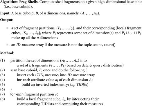
“How do we compute shell fragments of a data cube?” The shell fragment computation algorithm, Frag-Shells, is summarized in Figure 5.14. We first partition all the dimensions of the given data set into independent groups of dimensions, called fragments (line 1). We scan the base cuboid and construct an inverted index for each attribute (lines 2 to 6). Line 3 is for when the measure is other than the tuple count(), which will be described later. For each fragment, we compute the full local (i.e., fragment-based) data cube while retaining the inverted indices (lines 7 to 8). Consider a database of 60 dimensions, namely, A1, A2, …, A60. We can first partition the 60 dimensions into 20 fragments of size 3: (A1, A2, A3), (A4, A5, A6), …, (A58, A59, A60). For each fragment, we compute its full data cube while recording the inverted indices. For example, in fragment (A1, A2, A3), we would compute seven cuboids: A1, A2, A3, A1A2, A2A3, A1A3, A1A2A3. Furthermore, an inverted index is retained for each cell in the cuboids. That is, for each cell, its associated TID list is recorded.
The benefit of computing local cubes of each shell fragment instead of computing the complete cube shell can be seen by a simple calculation. For a base cuboid of 60 dimensions, there are only 7 × 20 = 140 cuboids to be computed according to the preceding shell fragment partitioning. This is in contrast to the 36,050 cuboids computed for the cube shell of size 3 described earlier! Notice that the above fragment partitioning is based simply on the grouping of consecutive dimensions. A more desirable approach would be to partition based on popular dimension groupings. This information can be obtained from domain experts or the past history of OLAP queries.
Let’s return to our running example to see how shell fragments are computed.
Example 5.10
Compute shell fragments
Suppose we are to compute the shell fragments of size 3. We first divide the five dimensions into two fragments, namely (A, B, C) and (D, E). For each fragment, we compute the full local data cube by intersecting the TID lists in Table 5.5 in a top-down depth-first order in the cuboid lattice. For example, to compute the cell (a1, b2, ∗), we intersect the TID lists of a1 and b2 to obtain a new list of {2, 3}. Cuboid AB is shown in Table 5.6.
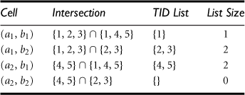
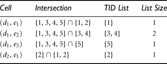
After computing cuboid AB, we can then compute cuboid ABC by intersecting all pairwise combinations between Table 5.6 and the row c1 in Table 5.5. Notice that because cell (a2, b2) is empty, it can be effectively discarded in subsequent computations, based on the Apriori property. The same process can be applied to compute fragment (D, E), which is completely independent from computing (A, B, C). Cuboid DE is shown in Table 5.7.
If the measure in the iceberg condition is count() (as in tuple counting), there is no need to reference the original database for this because the length of the TID list is equivalent to the tuple count. “Do we need to reference the original database if computing other measures such as average() ?” Actually, we can build and reference an ID_measure array instead, which stores what we need to compute other measures. For example, to compute average(), we let the ID_measure array hold three elements, namely, (TID, item_count, sum), for each cell (line 3 of the shell fragment computation algorithm in Figure 5.14). The average() measure for each aggregate cell can then be computed by accessing only this ID_measure array, using sum()/item_count(). Considering a database with 106 tuples, each taking 4 bytes each for TID, item_count, and sum, the ID_measure array requires 12 MB, whereas the corresponding database of 60 dimensions will require (60 + 3) × 4 × 106 = 252 MB (assuming each attribute value takes 4 bytes). Obviously, ID_measure array is a more compact data structure and is more likely to fit in memory than the corresponding high-dimensional database.
To illustrate the design of the ID_measure array, let’s look at Example 5.11.
Example 5.11
Computing cubes with the average() measure
Table 5.8 shows an example sales database where each tuple has two associated values, such as item_count and sum, where item_count is the count of items sold.
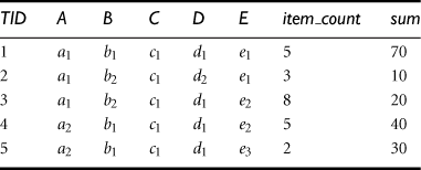
To compute a data cube for this database with the measure average(), we need to have a TID list for each cell: {TID1, …, TIDn}. Because each TID is uniquely associated with a particular set of measure values, all future computation just needs to fetch the measure values associated with the tuples in the list. In other words, by keeping an ID_measure array in memory for online processing, we can handle complex algebraic measures, such as average, variance, and standard deviation. Table 5.9 shows what exactly should be kept for our example, which is substantially smaller than the database itself.
The shell fragments are negligible in both storage space and computation time in comparison with the full data cube. Note that we can also use the Frag-Shells algorithm to compute the full data cube by including all the dimensions as a single fragment. Because the order of computation with respect to the cuboid lattice is top-down and depth-first (similar to that of BUC), the algorithm can perform Apriori pruning if applied to the construction of iceberg cubes.
“Once we have computed the shell fragments, how can they be used to answer OLAP queries?” Given the precomputed shell fragments, we can view the cube space as a virtual cube and perform OLAP queries related to the cube online. In general, two types of queries are possible: (1) point query and (2) subcube query.
In a point query, all of the relevant dimensions in the cube have been instantiated (i.e., there are no inquired dimensions in the relevant dimensions set). For example, in an n-dimensional data cube, A1A2…An, a point query could be in the form of ![]() , where A1 = {a11, a18}, A5 = {a52, a55, a59}, A9 = a94, and M is the inquired measure for each corresponding cube cell. For a cube with a small number of dimensions, we can use ∗ to represent a “don’t care” position where the corresponding dimension is irrelevant, that is, neither inquired nor instantiated. For example, in the query
, where A1 = {a11, a18}, A5 = {a52, a55, a59}, A9 = a94, and M is the inquired measure for each corresponding cube cell. For a cube with a small number of dimensions, we can use ∗ to represent a “don’t care” position where the corresponding dimension is irrelevant, that is, neither inquired nor instantiated. For example, in the query ![]() for the database in Table 5.4, the first four dimension values are instantiated to a2, b1, c1, and d1, respectively, while the last dimension is irrelevant, and count() (which is the tuple count by context) is the inquired measure.
for the database in Table 5.4, the first four dimension values are instantiated to a2, b1, c1, and d1, respectively, while the last dimension is irrelevant, and count() (which is the tuple count by context) is the inquired measure.
In a subcube query, at least one of the relevant dimensions in the cube is inquired. For example, in an n-dimensional data cube A1A2 … An, a subcube query could be in the form ![]() , where A1 = {a11, a18} and A9 = a94, A5 and A21 are the inquired dimensions, and M is the inquired measure. For a cube with a small number of dimensions, we can use ∗ for an irrelevant dimension and ? for an inquired one. For example, in the query
, where A1 = {a11, a18} and A9 = a94, A5 and A21 are the inquired dimensions, and M is the inquired measure. For a cube with a small number of dimensions, we can use ∗ for an irrelevant dimension and ? for an inquired one. For example, in the query ![]() we see that the first and third dimension values are instantiated to a2 and c1, respectively, while the fourth is irrelevant, and the second and the fifth are inquired. A subcube query computes all possible value combinations of the inquired dimensions. It essentially returns a local data cube consisting of the inquired dimensions.
we see that the first and third dimension values are instantiated to a2 and c1, respectively, while the fourth is irrelevant, and the second and the fifth are inquired. A subcube query computes all possible value combinations of the inquired dimensions. It essentially returns a local data cube consisting of the inquired dimensions.
“How can we use shell fragments to answer a point query?” Because a point query explicitly provides the instantiated variables set on the relevant dimensions set, we can make maximal use of the precomputed shell fragments by finding the best fitting (i.e., dimension-wise completely matching) fragments to fetch and intersect the associated TID lists.
Let the point query be of the form ![]() , where αi represents a set of instantiated values of dimension Ai, and so on for αj, αk, and αp. First, we check the shell fragment schema to determine which dimensions among Ai, Aj, Ak, and Ap are in the same fragment(s). Suppose Ai and Aj are in the same fragment, while Ak and Ap are in two other fragments. We fetch the corresponding TID lists on the precomputed 2-D fragment for dimensions Ai and Aj using the instantiations αi and αj, and fetch the TID lists on the 1-D fragments for dimensions Ak and Ap using the instantiations αk and αp, respectively. The obtained TID lists are intersected to derive the TID list table. This table is then used to derive the specified measure (e.g., by taking the length of the TID lists for tuple count(), or by fetching item_count() and sum() from the ID_measure array to compute average()) for the final set of cells.
, where αi represents a set of instantiated values of dimension Ai, and so on for αj, αk, and αp. First, we check the shell fragment schema to determine which dimensions among Ai, Aj, Ak, and Ap are in the same fragment(s). Suppose Ai and Aj are in the same fragment, while Ak and Ap are in two other fragments. We fetch the corresponding TID lists on the precomputed 2-D fragment for dimensions Ai and Aj using the instantiations αi and αj, and fetch the TID lists on the 1-D fragments for dimensions Ak and Ap using the instantiations αk and αp, respectively. The obtained TID lists are intersected to derive the TID list table. This table is then used to derive the specified measure (e.g., by taking the length of the TID lists for tuple count(), or by fetching item_count() and sum() from the ID_measure array to compute average()) for the final set of cells.
Example 5.12
Point query
Suppose a user wants to compute the point query ![]() for our database in Table 5.4 and that the shell fragments for the partitions (A, B, C) and (D, E) are precomputed as described in Example 5.10. The query is broken down into two subqueries based on the precomputed fragments:
for our database in Table 5.4 and that the shell fragments for the partitions (A, B, C) and (D, E) are precomputed as described in Example 5.10. The query is broken down into two subqueries based on the precomputed fragments: ![]() and
and ![]() . The best-fit precomputed shell fragments for the two subqueries are ABC and D. The fetch of the TID lists for the two subqueries returns two lists: {4, 5} and {1, 3, 4, 5}. Their intersection is the list {4, 5}, which is of size 2. Thus, the final answer is count() = 2.
. The best-fit precomputed shell fragments for the two subqueries are ABC and D. The fetch of the TID lists for the two subqueries returns two lists: {4, 5} and {1, 3, 4, 5}. Their intersection is the list {4, 5}, which is of size 2. Thus, the final answer is count() = 2.
“How can we use shell fragments to answer a subcube query?” A subcube query returns a local data cube based on the instantiated and inquired dimensions. Such a data cube needs to be aggregated in a multidimensional way so that online analytical processing (drilling, dicing, pivoting, etc.) can be made available to users for flexible manipulation and analysis. Because instantiated dimensions usually provide highly selective constants that dramatically reduce the size of the valid TID lists, we should make maximal use of the precomputed shell fragments by finding the fragments that best fit the set of instantiated dimensions, and fetching and intersecting the associated TID lists to derive the reduced TID list. This list can then be used to intersect the best-fitting shell fragments consisting of the inquired dimensions. This will generate the relevant and inquired base cuboid, which can then be used to compute the relevant subcube on-the-fly using an efficient online cubing algorithm.
Let the subcube query be of the form ![]() , where αi, αj, and αp represent a set of instantiated values of dimension Ai, Aj, and Ap, respectively, and Ak and Aq represent two inquired dimensions. First, we check the shell fragment schema to determine which dimensions among (1) Ai, Aj, and Ap, and (2) Ak and Aq are in the same fragment partition. Suppose Ai and Aj belong to the same fragment, as do Ak and Aq, but that Ap is in a different fragment. We fetch the corresponding TID lists in the precomputed 2-D fragment for Ai and Aj using the instantiations αi and αj, then fetch the TID list on the precomputed 1-D fragment for Ap using instantiation αp, and then fetch the TID lists on the precomputed 2-D fragments for Ak and Aq, respectively, using no instantiations (i.e., all possible values). The obtained TID lists are intersected to derive the final TID lists, which are used to fetch the corresponding measures from the ID_measure array to derive the “base cuboid” of a 2-D subcube for two dimensions (Ak, Aq). A fast cube computation algorithm can be applied to compute this 2-D cube based on the derived base cuboid. The computed 2-D cube is then ready for OLAP operations.
, where αi, αj, and αp represent a set of instantiated values of dimension Ai, Aj, and Ap, respectively, and Ak and Aq represent two inquired dimensions. First, we check the shell fragment schema to determine which dimensions among (1) Ai, Aj, and Ap, and (2) Ak and Aq are in the same fragment partition. Suppose Ai and Aj belong to the same fragment, as do Ak and Aq, but that Ap is in a different fragment. We fetch the corresponding TID lists in the precomputed 2-D fragment for Ai and Aj using the instantiations αi and αj, then fetch the TID list on the precomputed 1-D fragment for Ap using instantiation αp, and then fetch the TID lists on the precomputed 2-D fragments for Ak and Aq, respectively, using no instantiations (i.e., all possible values). The obtained TID lists are intersected to derive the final TID lists, which are used to fetch the corresponding measures from the ID_measure array to derive the “base cuboid” of a 2-D subcube for two dimensions (Ak, Aq). A fast cube computation algorithm can be applied to compute this 2-D cube based on the derived base cuboid. The computed 2-D cube is then ready for OLAP operations.
Example 5.13
Subcube query
Suppose that a user wants to compute the subcube query, ![]() , for our database shown earlier in Table 5.4, and that the shell fragments have been precomputed as described in Example 5.10. The query can be broken into three best-fit fragments according to the instantiated and inquired dimensions: AB, C, and E, where AB has the instantiation (a2, b1). The fetch of the TID lists for these partitions returns (a2, b1) : {4, 5}, (c1) : {1, 2, 3, 4, 5} and {(e1 : {1, 2}), (e2 : {3, 4}), (e3 : {5})}, respectively. The intersection of these corresponding TID lists contains a cuboid with two tuples: {(c1, e2) : {4},5 (c1, e3) : {5}}. This base cuboid can be used to compute the 2-D data cube, which is trivial.
, for our database shown earlier in Table 5.4, and that the shell fragments have been precomputed as described in Example 5.10. The query can be broken into three best-fit fragments according to the instantiated and inquired dimensions: AB, C, and E, where AB has the instantiation (a2, b1). The fetch of the TID lists for these partitions returns (a2, b1) : {4, 5}, (c1) : {1, 2, 3, 4, 5} and {(e1 : {1, 2}), (e2 : {3, 4}), (e3 : {5})}, respectively. The intersection of these corresponding TID lists contains a cuboid with two tuples: {(c1, e2) : {4},5 (c1, e3) : {5}}. This base cuboid can be used to compute the 2-D data cube, which is trivial.
5That is, the intersection of the TID lists for (a2, b1), (c1), and (e2) is {4}.
For large data sets, a fragment size of 2 or 3 typically results in reasonable storage requirements for the shell fragments and for fast query response time. Querying with shell fragments is substantially faster than answering queries using precomputed data cubes that are stored on disk. In comparison to full cube computation, Frag-Shells is recommended if there are less than four inquired dimensions. Otherwise, more efficient algorithms, such as Star-Cubing, can be used for fast online cube computation. Frag-Shells can be easily extended to allow incremental updates, the details of which are left as an exercise.