
3.5 Data Transformation and Data Discretization
This section presents methods of data transformation. In this preprocessing step, the data are transformed or consolidated so that the resulting mining process may be more efficient, and the patterns found may be easier to understand. Data discretization, a form of data transformation, is also discussed.
3.5.1 Data Transformation Strategies Overview
In data transformation, the data are transformed or consolidated into forms appropriate for mining. Strategies for data transformation include the following:
1. Smoothing, which works to remove noise from the data. Techniques include binning, regression, and clustering.
2. Attribute construction (or feature construction), where new attributes are constructed and added from the given set of attributes to help the mining process.
3. Aggregation, where summary or aggregation operations are applied to the data. For example, the daily sales data may be aggregated so as to compute monthly and annual total amounts. This step is typically used in constructing a data cube for data analysis at multiple abstraction levels.
4. Normalization, where the attribute data are scaled so as to fall within a smaller range, such as −1.0 to 1.0, or 0.0 to 1.0.
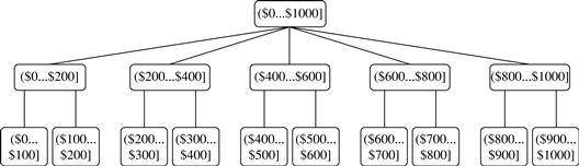
5. Discretization, where the raw values of a numeric attribute (e.g., age) are replaced by interval labels (e.g., 0–10, 11–20, etc.) or conceptual labels (e.g., youth, adult, senior). The labels, in turn, can be recursively organized into higher-level concepts, resulting in a concept hierarchy for the numeric attribute. Figure 3.12 shows a concept hierarchy for the attribute price. More than one concept hierarchy can be defined for the same attribute to accommodate the needs of various users.
6. Concept hierarchy generation for nominal data, where attributes such as street can be generalized to higher-level concepts, like city or country. Many hierarchies for nominal attributes are implicit within the database schema and can be automatically defined at the schema definition level.
Recall that there is much overlap between the major data preprocessing tasks. The first three of these strategies were discussed earlier in this chapter. Smoothing is a form of data cleaning and was addressed in Section 3.2.2. Section 3.2.3 on the data cleaning process also discussed ETL tools, where users specify transformations to correct data inconsistencies. Attribute construction and aggregation were discussed in Section 3.4 on data reduction. In this section, we therefore concentrate on the latter three strategies.
Discretization techniques can be categorized based on how the discretization is performed, such as whether it uses class information or which direction it proceeds (i.e., top-down vs. bottom-up). If the discretization process uses class information, then we say it is supervised discretization. Otherwise, it is unsupervised. If the process starts by first finding one or a few points (called split points or cut points) to split the entire attribute range, and then repeats this recursively on the resulting intervals, it is called top-down discretization or splitting. This contrasts with bottom-up discretization or merging, which starts by considering all of the continuous values as potential split-points, removes some by merging neighborhood values to form intervals, and then recursively applies this process to the resulting intervals.
Data discretization and concept hierarchy generation are also forms of data reduction. The raw data are replaced by a smaller number of interval or concept labels. This simplifies the original data and makes the mining more efficient. The resulting patterns mined are typically easier to understand. Concept hierarchies are also useful for mining at multiple abstraction levels.
The rest of this section is organized as follows. First, normalization techniques are presented in Section 3.5.2. We then describe several techniques for data discretization, each of which can be used to generate concept hierarchies for numeric attributes. The techniques include binning (Section 3.5.3) and histogram analysis (Section 3.5.4), as well as cluster analysis, decision tree analysis, and correlation analysis (Section 3.5.5). Finally, Section 3.5.6 describes the automatic generation of concept hierarchies for nominal data.
3.5.2 Data Transformation by Normalization
The measurement unit used can affect the data analysis. For example, changing measurement units from meters to inches for height, or from kilograms to pounds for weight, may lead to very different results. In general, expressing an attribute in smaller units will lead to a larger range for that attribute, and thus tend to give such an attribute greater effect or “weight.” To help avoid dependence on the choice of measurement units, the data should be normalized or standardized. This involves transforming the data to fall within a smaller or common range such as [−1, 1] or [0.0, 1.0]. (The terms standardize and normalize are used interchangeably in data preprocessing, although in statistics, the latter term also has other connotations.)
Normalizing the data attempts to give all attributes an equal weight. Normalization is particularly useful for classification algorithms involving neural networks or distance measurements such as nearest-neighbor classification and clustering. If using the neural network backpropagation algorithm for classification mining (Chapter 9), normalizing the input values for each attribute measured in the training tuples will help speed up the learning phase. For distance-based methods, normalization helps prevent attributes with initially large ranges (e.g., income) from outweighing attributes with initially smaller ranges (e.g., binary attributes). It is also useful when given no prior knowledge of the data.
There are many methods for data normalization. We study min-max normalization, z-score normalization, and normalization by decimal scaling. For our discussion, let A be a numeric attribute with n observed values, v1, v2, …, vn.
Min-max normalization performs a linear transformation on the original data. Suppose that minA and maxA are the minimum and maximum values of an attribute, A. Min-max normalization maps a value, vi, of A to v′i in the range [new_minA, new_maxA] by computing
![]() (3.8)
(3.8)
Min-max normalization preserves the relationships among the original data values. It will encounter an “out-of-bounds” error if a future input case for normalization falls outside of the original data range for A.
Example 3.4
Min-max normalization
Suppose that the minimum and maximum values for the attribute income are $12,000 and $98,000, respectively. We would like to map income to the range [0.0, 1.0]. By min-max normalization, a value of $73,600 for income is transformed to ![]() .
.
In z -score normalization (or zero-mean normalization), the values for an attribute, A, are normalized based on the mean (i.e., average) and standard deviation of A. A value, vi, of A is normalized to v′i by computing
![]() (3.9)
(3.9)
where Ā and σA are the mean and standard deviation, respectively, of attribute A. The mean and standard deviation were discussed in Section 2.2, where ![]() and σA is computed as the square root of the variance of A (see Eq. (2.6)). This method of normalization is useful when the actual minimum and maximum of attribute A are unknown, or when there are outliers that dominate the min-max normalization.
and σA is computed as the square root of the variance of A (see Eq. (2.6)). This method of normalization is useful when the actual minimum and maximum of attribute A are unknown, or when there are outliers that dominate the min-max normalization.
Example 3.5
z-score normalization
Suppose that the mean and standard deviation of the values for the attribute income are $54,000 and $16,000, respectively. With z-score normalization, a value of $73,600 for income is transformed to ![]() .
.
A variation of this z-score normalization replaces the standard deviation of Eq. (3.9) by the mean absolute deviation of A. The mean absolute deviation of A, denoted sA, is
![]() (3.10)
(3.10)
Thus, z-score normalization using the mean absolute deviation is
![]() (3.11)
(3.11)
The mean absolute deviation, sA, is more robust to outliers than the standard deviation, σA. When computing the mean absolute deviation, the deviations from the mean (i.e., ![]() ) are not squared; hence, the effect of outliers is somewhat reduced.
) are not squared; hence, the effect of outliers is somewhat reduced.
Normalization by decimal scaling normalizes by moving the decimal point of values of attribute A. The number of decimal points moved depends on the maximum absolute value of A. A value, vi, of A is normalized to v′i by computing
![]() (3.12)
(3.12)
where j is the smallest integer such that max(|v′i|) < 1.
Note that normalization can change the original data quite a bit, especially when using z-score normalization or decimal scaling. It is also necessary to save the normalization parameters (e.g., the mean and standard deviation if using z-score normalization) so that future data can be normalized in a uniform manner.
3.5.3 Discretization by Binning
Binning is a top-down splitting technique based on a specified number of bins. Section 3.2.2 discussed binning methods for data smoothing. These methods are also used as discretization methods for data reduction and concept hierarchy generation. For example, attribute values can be discretized by applying equal-width or equal-frequency binning, and then replacing each bin value by the bin mean or median, as in smoothing by bin means or smoothing by bin medians, respectively. These techniques can be applied recursively to the resulting partitions to generate concept hierarchies.
Binning does not use class information and is therefore an unsupervised discretization technique. It is sensitive to the user-specified number of bins, as well as the presence of outliers.
3.5.4 Discretization by Histogram Analysis
Like binning, histogram analysis is an unsupervised discretization technique because it does not use class information. Histograms were introduced in Section 2.2.3. A histogram partitions the values of an attribute, A, into disjoint ranges called buckets or bins.
Various partitioning rules can be used to define histograms (Section 3.4.6). In an equal-width histogram, for example, the values are partitioned into equal-size partitions or ranges (e.g., earlier in Figure 3.8 for price, where each bucket has a width of $10). With an equal-frequency histogram, the values are partitioned so that, ideally, each partition contains the same number of data tuples. The histogram analysis algorithm can be applied recursively to each partition in order to automatically generate a multilevel concept hierarchy, with the procedure terminating once a prespecified number of concept levels has been reached. A minimum interval size can also be used per level to control the recursive procedure. This specifies the minimum width of a partition, or the minimum number of values for each partition at each level. Histograms can also be partitioned based on cluster analysis of the data distribution, as described next.
3.5.5 Discretization by Cluster, Decision Tree, and Correlation Analyses
Clustering, decision tree analysis, and correlation analysis can be used for data discretization. We briefly study each of these approaches.
Cluster analysis is a popular data discretization method. A clustering algorithm can be applied to discretize a numeric attribute, A, by partitioning the values of A into clusters or groups. Clustering takes the distribution of A into consideration, as well as the closeness of data points, and therefore is able to produce high-quality discretization results.
Clustering can be used to generate a concept hierarchy for A by following either a top-down splitting strategy or a bottom-up merging strategy, where each cluster forms a node of the concept hierarchy. In the former, each initial cluster or partition may be further decomposed into several subclusters, forming a lower level of the hierarchy. In the latter, clusters are formed by repeatedly grouping neighboring clusters in order to form higher-level concepts. Clustering methods for data mining are studied in Chapters 10 and 11.
Techniques to generate decision trees for classification (Chapter 8) can be applied to discretization. Such techniques employ a top-down splitting approach. Unlike the other methods mentioned so far, decision tree approaches to discretization are supervised, that is, they make use of class label information. For example, we may have a data set of patient symptoms (the attributes) where each patient has an associated diagnosis class label. Class distribution information is used in the calculation and determination of split-points (data values for partitioning an attribute range). Intuitively, the main idea is to select split-points so that a given resulting partition contains as many tuples of the same class as possible. Entropy is the most commonly used measure for this purpose. To discretize a numeric attribute, A, the method selects the value of A that has the minimum entropy as a split-point, and recursively partitions the resulting intervals to arrive at a hierarchical discretization. Such discretization forms a concept hierarchy for A.
Because decision tree–based discretization uses class information, it is more likely that the interval boundaries (split-points) are defined to occur in places that may help improve classification accuracy. Decision trees and the entropy measure are described in greater detail in Section 8.2.2.
Measures of correlation can be used for discretization. ChiMerge is a χ2-based discretization method. The discretization methods that we have studied up to this point have all employed a top-down, splitting strategy. This contrasts with ChiMerge, which employs a bottom-up approach by finding the best neighboring intervals and then merging them to form larger intervals, recursively. As with decision tree analysis, ChiMerge is supervised in that it uses class information. The basic notion is that for accurate discretization, the relative class frequencies should be fairly consistent within an interval. Therefore, if two adjacent intervals have a very similar distribution of classes, then the intervals can be merged. Otherwise, they should remain separate.
ChiMerge proceeds as follows. Initially, each distinct value of a numeric attribute A is considered to be one interval. χ2 tests are performed for every pair of adjacent intervals. Adjacent intervals with the least χ2 values are merged together, because low χ2 values for a pair indicate similar class distributions. This merging process proceeds recursively until a predefined stopping criterion is met.
3.5.6 Concept Hierarchy Generation for Nominal Data
We now look at data transformation for nominal data. In particular, we study concept hierarchy generation for nominal attributes. Nominal attributes have a finite (but possibly large) number of distinct values, with no ordering among the values. Examples include geographic_location, job_category, and item_type.
Manual definition of concept hierarchies can be a tedious and time-consuming task for a user or a domain expert. Fortunately, many hierarchies are implicit within the database schema and can be automatically defined at the schema definition level. The concept hierarchies can be used to transform the data into multiple levels of granularity. For example, data mining patterns regarding sales may be found relating to specific regions or countries, in addition to individual branch locations.
We study four methods for the generation of concept hierarchies for nominal data, as follows.
1. Specification of a partial ordering of attributes explicitly at the schema level by users or experts: Concept hierarchies for nominal attributes or dimensions typically involve a group of attributes. A user or expert can easily define a concept hierarchy by specifying a partial or total ordering of the attributes at the schema level. For example, suppose that a relational database contains the following group of attributes: street, city, province_or_state, and country. Similarly, a data warehouse location dimension may contain the same attributes. A hierarchy can be defined by specifying the total ordering among these attributes at the schema level such as street < city < province_or_state < country.
2. Specification of a portion of a hierarchy by explicit data grouping: This is essentially the manual definition of a portion of a concept hierarchy. In a large database, it is unrealistic to define an entire concept hierarchy by explicit value enumeration. On the contrary, we can easily specify explicit groupings for a small portion of intermediate-level data. For example, after specifying that province and country form a hierarchy at the schema level, a user could define some intermediate levels manually, such as “{Alberta, Saskatchewan, Manitoba} ⊂ prairies_Canada” and “{British Columbia, prairies_Canada} ⊂ Western_Canada.”
3. Specification of a set of attributes, but not of their partial ordering: A user may specify a set of attributes forming a concept hierarchy, but omit to explicitly state their partial ordering. The system can then try to automatically generate the attribute ordering so as to construct a meaningful concept hierarchy.
“Without knowledge of data semantics, how can a hierarchical ordering for an arbitrary set of nominal attributes be found?” Consider the observation that since higher-level concepts generally cover several subordinate lower-level concepts, an attribute defining a high concept level (e.g., country) will usually contain a smaller number of distinct values than an attribute defining a lower concept level (e.g., street). Based on this observation, a concept hierarchy can be automatically generated based on the number of distinct values per attribute in the given attribute set. The attribute with the most distinct values is placed at the lowest hierarchy level. The lower the number of distinct values an attribute has, the higher it is in the generated concept hierarchy. This heuristic rule works well in many cases. Some local-level swapping or adjustments may be applied by users or experts, when necessary, after examination of the generated hierarchy.
Let’s examine an example of this third method.
Example 3.7
Concept hierarchy generation based on the number of distinct values per attribute
Suppose a user selects a set of location-oriented attributes—street, country, province_ or_state, and city —from the AllElectronics database, but does not specify the hierarchical ordering among the attributes.
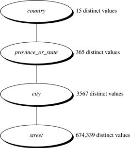
A concept hierarchy for location can be generated automatically, as illustrated in Figure 3.13. First, sort the attributes in ascending order based on the number of distinct values in each attribute. This results in the following (where the number of distinct values per attribute is shown in parentheses): country (15), province_or_state (365), city (3567), and street (674,339). Second, generate the hierarchy from the top down according to the sorted order, with the first attribute at the top level and the last attribute at the bottom level. Finally, the user can examine the generated hierarchy, and when necessary, modify it to reflect desired semantic relationships among the attributes. In this example, it is obvious that there is no need to modify the generated hierarchy.
Note that this heuristic rule is not foolproof. For example, a time dimension in a database may contain 20 distinct years, 12 distinct months, and 7 distinct days of the week. However, this does not suggest that the time hierarchy should be “year < month < days_of_the_week,” with days_of_the_week at the top of the hierarchy.
4. Specification of only a partial set of attributes: Sometimes a user can be careless when defining a hierarchy, or have only a vague idea about what should be included in a hierarchy. Consequently, the user may have included only a small subset of the relevant attributes in the hierarchy specification. For example, instead of including all of the hierarchically relevant attributes for location, the user may have specified only street and city. To handle such partially specified hierarchies, it is important to embed data semantics in the database schema so that attributes with tight semantic connections can be pinned together. In this way, the specification of one attribute may trigger a whole group of semantically tightly linked attributes to be “dragged in” to form a complete hierarchy. Users, however, should have the option to override this feature, as necessary.
In summary, information at the schema level and on attribute–value counts can be used to generate concept hierarchies for nominal data. Transforming nominal data with the use of concept hierarchies allows higher-level knowledge patterns to be found. It allows mining at multiple levels of abstraction, which is a common requirement for data mining applications.