
11.2 Clustering High-Dimensional Data
The clustering methods we have studied so far work well when the dimensionality is not high, that is, having less than 10 attributes. There are, however, important applications of high dimensionality. “How can we conduct cluster analysis on high-dimensional data?”
In this section, we study approaches to clustering high-dimensional data. Section 11.2.1 starts with an overview of the major challenges and the approaches used. Methods for high-dimensional data clustering can be divided into two categories: subspace clustering methods (Section 11.2.2 and 11.2.3) and dimensionality reduction methods (Section 11.2.4).
11.2.1 Clustering High-Dimensional Data: Problems, Challenges, and Major Methodologies
Before we present any specific methods for clustering high-dimensional data, let’s first demonstrate the needs of cluster analysis on high-dimensional data using examples. We examine the challenges that call for new methods. We then categorize the major methods according to whether they search for clusters in subspaces of the original space, or whether they create a new lower-dimensionality space and search for clusters there.
In some applications, a data object may be described by 10 or more attributes. Such objects are referred to as a high-dimensional data space.
Example 11.9
High-dimensional data and clustering
AllElectronics keeps track of the products purchased by every customer. As a customer-relationship manager, you want to cluster customers into groups according to what they purchased from AllElectronics.
The customer purchase data are of very high dimensionality. AllElectronics carries tens of thousands of products. Therefore, a customer’s purchase profile, which is a vector of the products carried by the company, has tens of thousands of dimensions.
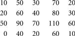
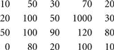
“Are the traditional distance measures, which are frequently used in low-dimensional cluster analysis, also effective on high-dimensional data?” Consider the customers in Table 11.4, where 10 products, P1, …, P10, are used in demonstration. If a customer purchases a product, a 1 is set at the corresponding bit; otherwise, a 0 appears. Let’s calculate the Euclidean distances (Eq. 2.16) among Ada, Bob, and Cathy. It is easy to see that
![]()
According to Euclidean distance, the three customers are equivalently similar (or dissimilar) to each other. However, a close look tells us that Ada should be more similar to Cathy than to Bob because Ada and Cathy share one common purchased item, P1.

As shown in Example 11.9, the traditional distance measures can be ineffective on high-dimensional data. Such distance measures may be dominated by the noise in many dimensions. Therefore, clusters in the full, high-dimensional space can be unreliable, and finding such clusters may not be meaningful.
“Then what kinds of clusters are meaningful on high-dimensional data?” For cluster analysis of high-dimensional data, we still want to group similar objects together. However, the data space is often too big and too messy. An additional challenge is that we need to find not only clusters, but, for each cluster, a set of attributes that manifest the cluster. In other words, a cluster on high-dimensional data often is defined using a small set of attributes instead of the full data space. Essentially, clustering high-dimensional data should return groups of objects as clusters (as conventional cluster analysis does), in addition to, for each cluster, the set of attributes that characterize the cluster. For example, in Table 11.4, to characterize the similarity between Ada and Cathy, P1 may be returned as the attribute because Ada and Cathy both purchased P1.
Clustering high-dimensional data is the search for clusters and the space in which they exist. Thus, there are two major kinds of methods:
■ Subspace clustering approaches search for clusters existing in subspaces of the given high-dimensional data space, where a subspace is defined using a subset of attributes in the full space. Subspace clustering approaches are discussed in Section 11.2.2.
■ Dimensionality reduction approaches try to construct a much lower-dimensional space and search for clusters in such a space. Often, a method may construct new dimensions by combining some dimensions from the original data. Dimensionality reduction methods are the topic of Section 11.2.4.
In general, clustering high-dimensional data raises several new challenges in addition to those of conventional clustering:
■ A major issue is how to create appropriate models for clusters in high-dimensional data. Unlike conventional clusters in low-dimensional spaces, clusters hidden in high-dimensional data are often significantly smaller. For example, when clustering customer-purchase data, we would not expect many users to have similar purchase patterns. Searching for such small but meaningful clusters is like finding needles in a haystack. As shown before, the conventional distance measures can be ineffective. Instead, we often have to consider various more sophisticated techniques that can model correlations and consistency among objects in subspaces.
■ There are typically an exponential number of possible subspaces or dimensionality reduction options, and thus the optimal solutions are often computationally prohibitive. For example, if the original data space has 1000 dimensions, and we want to find clusters of dimensionality 10, then there are ![]() possible subspaces.
possible subspaces.
11.2.2 Subspace Clustering Methods
“How can we find subspace clusters from high-dimensional data?” Many methods have been proposed. They generally can be categorized into three major groups: subspace search methods, correlation-based clustering methods, and biclustering methods.
Subspace Search Methods
A subspace search method searches various subspaces for clusters. Here, a cluster is a subset of objects that are similar to each other in a subspace. The similarity is often captured by conventional measures such as distance or density. For example, the CLIQUE algorithm introduced in Section 10.5.2 is a subspace clustering method. It enumerates subspaces and the clusters in those subspaces in a dimensionality-increasing order, and applies antimonotonicity to prune subspaces in which no cluster may exist.
A major challenge that subspace search methods face is how to search a series of subspaces effectively and efficiently. Generally there are two kinds of strategies:
■ Bottom-up approaches start from low-dimensional subspaces and search higher-dimensional subspaces only when there may be clusters in those higher-dimensional subspaces. Various pruning techniques are explored to reduce the number of higher-dimensional subspaces that need to be searched. CLIQUE is an example of a bottom-up approach.
■ Top-down approaches start from the full space and search smaller and smaller subspaces recursively. Top-down approaches are effective only if the locality assumption holds, which require that the subspace of a cluster can be determined by the local neighborhood.
Correlation-Based Clustering Methods
While subspace search methods search for clusters with a similarity that is measured using conventional metrics like distance or density, correlation-based approaches can further discover clusters that are defined by advanced correlation models.
For additional details on subspace search methods and correlation-based clustering methods, please refer to the bibliographic notes (Section 11.7).
Biclustering Methods
In some applications, we want to cluster both objects and attributes simultaneously. The resulting clusters are known as biclusters and meet four requirements: (1) only a small set of objects participate in a cluster; (2) a cluster only involves a small number of attributes; (3) an object may participate in multiple clusters, or does not participate in any cluster; and (4) an attribute may be involved in multiple clusters, or is not involved in any cluster. Section 11.2.3 discusses biclustering in detail.
11.2.3 Biclustering
In the cluster analysis discussed so far, we cluster objects according to their attribute values. Objects and attributes are not treated in the same way. However, in some applications, objects and attributes are defined in a symmetric way, where data analysis involves searching data matrices for submatrices that show unique patterns as clusters. This kind of clustering technique belongs to the category of biclustering.
This section first introduces two motivating application examples of biclustering–gene expression and recommender systems. You will then learn about the different types of biclusters. Last, we present biclustering methods.
Application Examples
Biclustering techniques were first proposed to address the needs for analyzing gene expression data. A gene is a unit of the passing-on of traits from a living organism to its offspring. Typically, a gene resides on a segment of DNA. Genes are critical for all living things because they specify all proteins and functional RNA chains. They hold the information to build and maintain a living organism’s cells and pass genetic traits to offspring. Synthesis of a functional gene product, either RNA or protein, relies on the process of gene expression. A genotype is the genetic makeup of a cell, an organism, or an individual. Phenotypes are observable characteristics of an organism. Gene expression is the most fundamental level in genetics in that genotypes cause phenotypes.
Using DNA chips (also known as DNA microarrays ) and other biological engineering techniques, we can measure the expression level of a large number (possibly all) of an organism’s genes, in a number of different experimental conditions. Such conditions may correspond to different time points in an experiment or samples from different organs. Roughly speaking, the gene expression data or DNA microarray data are conceptually a gene-sample/condition matrix, where each row corresponds to one gene, and each column corresponds to one sample or condition. Each element in the matrix is a real number and records the expression level of a gene under a specific condition. Figure 11.3 shows an illustration.
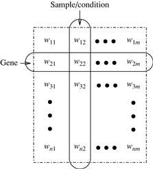
From the clustering viewpoint, an interesting issue is that a gene expression data matrix can be analyzed in two dimensions—the gene dimension and the sample/ condition dimension.
■ When analyzing in the gene dimension, we treat each gene as an object and treat the samples/conditions as attributes. By mining in the gene dimension, we may find patterns shared by multiple genes, or cluster genes into groups. For example, we may find a group of genes that express themselves similarly, which is highly interesting in bioinformatics, such as in finding pathways.
■ When analyzing in the sample/condition dimension, we treat each sample/condition as an object and treat the genes as attributes. In this way, we may find patterns of samples/conditions, or cluster samples/conditions into groups. For example, we may find the differences in gene expression by comparing a group of tumor samples and nontumor samples.
As can be seen, many gene expression data mining problems are highly related to cluster analysis. However, a challenge here is that, instead of clustering in one dimension (e.g., gene or sample/condition), in many cases we need to cluster in two dimensions simultaneously (e.g., both gene and sample/condition). Moreover, unlike the clustering models we have discussed so far, a cluster in a gene expression data matrix is a submatrix and usually has the following characteristics:
■ Only a small set of genes participate in the cluster.
■ The cluster involves only a small subset of samples/conditions.
■ A gene may participate in multiple clusters, or may not participate in any cluster.
■ A sample/condition may be involved in multiple clusters, or may not be involved in any cluster.
To find clusters in gene-sample/condition matrices, we need new clustering techniques that meet the following requirements for biclustering:
■ A cluster of genes is defined using only a subset of samples/conditions.
■ A cluster of samples/conditions is defined using only a subset of genes.
■ The clusters are neither exclusive (e.g., where one gene can participate in multiple clusters) nor exhaustive (e.g., where a gene may not participate in any cluster).
Biclustering is useful not only in bioinformatics, but also in other applications as well. Consider recommender systems as an example.
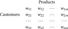
As with biclusters in a gene expression data matrix, the biclusters in a customer-product matrix usually have the following characteristics:
■ Only a small set of customers participate in a cluster.
■ A cluster involves only a small subset of products.
■ A customer can participate in multiple clusters, or may not participate in any cluster.
■ A product may be involved in multiple clusters, or may not be involved in any cluster.
Biclustering can be applied to customer-product matrices to mine clusters satisfying these requirements.
11.2.3 Types of Biclusters
“How can we model biclusters and mine them?” Let’s start with some basic notation. For the sake of simplicity, we will use “genes” and “conditions” to refer to the two dimensions in our discussion. Our discussion can easily be extended to other applications. For example, we can simply replace “genes” and “conditions” by “customers” and “products” to tackle the customer-product biclustering problem.
Let ![]() be a set of genes and
be a set of genes and ![]() be a set of conditions. Let
be a set of conditions. Let ![]() be a gene expression data matrix, that is, a gene-condition matrix, where
be a gene expression data matrix, that is, a gene-condition matrix, where ![]() and
and ![]() . A submatrix I × J is defined by a subset
. A submatrix I × J is defined by a subset ![]() of genes and a subset
of genes and a subset ![]() of conditions. For example, in the matrix shown in Figure 11.5,
of conditions. For example, in the matrix shown in Figure 11.5, ![]() is a submatrix.
is a submatrix.
A bicluster is a submatrix where genes and conditions follow consistent patterns. We can define different types of biclusters based on such patterns.
■ As the simplest case, a submatrix I × J![]() is a bicluster with constant values if for any
is a bicluster with constant values if for any ![]() and
and ![]() ,
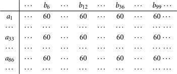
, ![]() , where c is a constant. For example, the submatrix
, where c is a constant. For example, the submatrix ![]() in Figure 11.5 is a bicluster with constant values.
in Figure 11.5 is a bicluster with constant values.
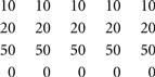
■ A bicluster is interesting if each row has a constant value, though different rows may have different values. A bicluster with constant values on rows is a submatrix I × J such that for any ![]() and
and ![]() ,
, ![]() , where αi is the adjustment for row i. For example, Figure 11.6 shows a bicluster with constant values on rows.
, where αi is the adjustment for row i. For example, Figure 11.6 shows a bicluster with constant values on rows.
Symmetrically, a bicluster with constant values on columns is a submatrix I × J such that for any ![]() and
and ![]() ,
, ![]() , where βj is the adjustment for column j.
, where βj is the adjustment for column j.
■ More generally, a bicluster is interesting if the rows change in a synchronized way with respect to the columns and vice versa. Mathematically, a bicluster with coherent values (also known as a pattern-based cluster ) is a submatrix I × J such that for any ![]() and
and ![]() ,
, ![]() , where αi and βj are the adjustment for row i and column j, respectively. For example, Figure 11.7 shows a bicluster with coherent values.
, where αi and βj are the adjustment for row i and column j, respectively. For example, Figure 11.7 shows a bicluster with coherent values.
It can be shown that I × J is a bicluster with coherent values if and only if for any ![]() and
and ![]() , then
, then ![]() . Moreover, instead of using addition, we can define a bicluster with coherent values using multiplication, that is,
. Moreover, instead of using addition, we can define a bicluster with coherent values using multiplication, that is, ![]() . Clearly, biclusters with constant values on rows or columns are special cases of biclusters with coherent values.
. Clearly, biclusters with constant values on rows or columns are special cases of biclusters with coherent values.
■ In some applications, we may only be interested in the up- or down-regulated changes across genes or conditions without constraining the exact values. A bicluster with coherent evolutions on rows is a submatrix I × J such that for any ![]() and
and ![]() ,
, ![]() . For example, Figure 11.8 shows a bicluster with coherent evolutions on rows. Symmetrically, we can define biclusters with coherent evolutions on columns.
. For example, Figure 11.8 shows a bicluster with coherent evolutions on rows. Symmetrically, we can define biclusters with coherent evolutions on columns.
Next, we study how to mine biclusters.
Biclustering Methods
The previous specification of the types of biclusters only considers ideal cases. In real data sets, such perfect biclusters rarely exist. When they do exist, they are usually very small. Instead, random noise can affect the readings of eij and thus prevent a bicluster in nature from appearing in a perfect shape.
There are two major types of methods for discovering biclusters in data that may come with noise. Optimization-based methods conduct an iterative search. At each iteration, the submatrix with the highest significance score is identified as a bicluster. The process terminates when a user-specified condition is met. Due to cost concerns in computation, greedy search is often employed to find local optimal biclusters. Enumeration methods use a tolerance threshold to specify the degree of noise allowed in the biclusters to be mined, and then tries to enumerate all submatrices of biclusters that satisfy the requirements. We use the δ-Cluster and MaPle algorithms as examples to illustrate these ideas.
Optimization Using the δ-Cluster Algorithm
For a submatrix, I × J, the mean of the i th row is
![]() (11.16)
(11.16)
Symmetrically, the mean of the j th column is
![]() (11.17)
(11.17)
The mean of all elements in the submatrix is
![]() (11.18)
(11.18)
The quality of the submatrix as a bicluster can be measured by the mean-squared residue value as
![]() (11.19)
(11.19)
Submatrix I × J is a δ-bicluster if ![]() , where
, where ![]() is a threshold. When
is a threshold. When ![]() , I × J is a perfect bicluster with coherent values. By setting
, I × J is a perfect bicluster with coherent values. By setting ![]() , a user can specify the tolerance of average noise per element against a perfect bicluster, because in Eq. (11.19) the residue on each element is
, a user can specify the tolerance of average noise per element against a perfect bicluster, because in Eq. (11.19) the residue on each element is
![]() (11.20)
(11.20)
A maximal δ-bicluster is a δ-bicluster I × J such that there does not exist another δ-bicluster ![]() , and
, and ![]() ,
, ![]() , and at least one inequality holds. Finding the maximal δ-bicluster of the largest size is computationally costly. Therefore, we can use a heuristic greedy search method to obtain a local optimal cluster. The algorithm works in two phases.
, and at least one inequality holds. Finding the maximal δ-bicluster of the largest size is computationally costly. Therefore, we can use a heuristic greedy search method to obtain a local optimal cluster. The algorithm works in two phases.
■ In the deletion phase, we start from the whole matrix. While the mean-squared residue of the matrix is over δ, we iteratively remove rows and columns. At each iteration, for each row i, we compute the mean-squared residue as
![]() (11.21)
(11.21)
Moreover, for each column j, we compute the mean-squared residue as
![]() (11.22)
(11.22)
We remove the row or column of the largest mean-squared residue. At the end of this phase, we obtain a submatrix I × J that is a δ-bicluster. However, the submatrix may not be maximal.
■ In the addition phase, we iteratively expand the δ-bicluster I × J obtained in the deletion phase as long as the δ-bicluster requirement is maintained. At each iteration, we consider rows and columns that are not involved in the current bicluster I × J by calculating their mean-squared residues. A row or column of the smallest mean-squared residue is added into the current δ-bicluster.
This greedy algorithm can find one δ-bicluster only. To find multiple biclusters that do not have heavy overlaps, we can run the algorithm multiple times. After each execution where a δ-bicluster is output, we can replace the elements in the output bicluster by random numbers. Although the greedy algorithm may find neither the optimal biclusters nor all biclusters, it is very fast even on large matrices.
Enumerating All Biclusters Using MaPle
As mentioned, a submatrix I × J is a bicluster with coherent values if and only if for any ![]() and
and ![]() ,
, ![]() . For any
. For any ![]() submatrix of I × J, we can define a p-score as
submatrix of I × J, we can define a p-score as
![]() (11.23)
(11.23)
A submatrix I × J is a δ-pCluster (for p attern-based cluster ) if the p-score of every ![]() submatrix of I × J is at most δ, where
submatrix of I × J is at most δ, where ![]() is a threshold specifying a user’s tolerance of noise against a perfect bicluster. Here, the p-score controls the noise on every element in a bicluster, while the mean-squared residue captures the average noise.
is a threshold specifying a user’s tolerance of noise against a perfect bicluster. Here, the p-score controls the noise on every element in a bicluster, while the mean-squared residue captures the average noise.
An interesting property of δ-pCluster is that if I × J is a δ-pCluster, then every x × y (x, y ≥ 2) submatrix of I × J is also a δ-pCluster. This monotonicity enables us to obtain a succinct representation of nonredundant δ-pClusters. A δ-pCluster is maximal if no more rows or columns can be added into the cluster while maintaining the δ-pCluster property. To avoid redundancy, instead of finding all δ-pClusters, we only need to compute all maximal δ-pClusters.
MaPle is an algorithm that enumerates all maximal δ-pClusters. It systematically enumerates every combination of conditions using a set enumeration tree and a depth-first search. This enumeration framework is the same as the pattern-growth methods for frequent pattern mining (Chapter 6). Consider gene expression data. For each condition combination, J, MaPle finds the maximal subsets of genes, I, such that I × J is a δ-pCluster. If I × J is not a submatrix of another δ-pCluster, then I × J is a maximal δ-pCluster.
There may be a huge number of condition combinations. MaPle prunes many unfruitful combinations using the monotonicity of δ-pClusters. For a condition combination, J, if there does not exist a set of genes, I, such that I × J is a δ-pCluster, then we do not need to consider any superset of J. Moreover, we should consider I × J as a candidate of a δ-pCluster only if for every ![]() -subset J′ of J,
-subset J′ of J, ![]() is a δ-pCluster. MaPle also employs several pruning techniques to speed up the search while retaining the completeness of returning all maximal δ-pClusters. For example, when examining a current δ-pCluster, I × J, MaPle collects all the genes and conditions that may be added to expand the cluster. If these candidate genes and conditions together with I and J form a submatrix of a δ-pCluster that has already been found, then the search of I × J and any superset of J can be pruned. Interested readers may refer to the bibliographic notes for additional information on the MaPle algorithm (Section 11.7).
is a δ-pCluster. MaPle also employs several pruning techniques to speed up the search while retaining the completeness of returning all maximal δ-pClusters. For example, when examining a current δ-pCluster, I × J, MaPle collects all the genes and conditions that may be added to expand the cluster. If these candidate genes and conditions together with I and J form a submatrix of a δ-pCluster that has already been found, then the search of I × J and any superset of J can be pruned. Interested readers may refer to the bibliographic notes for additional information on the MaPle algorithm (Section 11.7).
An interesting observation here is that the search for maximal δ-pClusters in MaPle is somewhat similar to mining frequent closed itemsets. Consequently, MaPle borrows the depth-first search framework and ideas from the pruning techniques of pattern-growth methods for frequent pattern mining. This is an example where frequent pattern mining and cluster analysis may share similar techniques and ideas.
An advantage of MaPle and the other algorithms that enumerate all biclusters is that they guarantee the completeness of the results and do not miss any overlapping biclusters. However, a challenge for such enumeration algorithms is that they may become very time consuming if a matrix becomes very large, such as a customer-purchase matrix of hundreds of thousands of customers and millions of products.
11.2.4 Dimensionality Reduction Methods and Spectral Clustering
Subspace clustering methods try to find clusters in subspaces of the original data space. In some situations, it is more effective to construct a new space instead of using subspaces of the original data. This is the motivation behind dimensionality reduction methods for clustering high-dimensional data.
Example 11.14
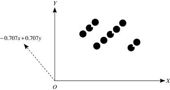
Clustering in a derived space
Consider the three clusters of points in Figure 11.9. It is not possible to cluster these points in any subspace of the original space, X × Y, because all three clusters would end up being projected onto overlapping areas in the x and y axes. What if, instead, we construct a new dimension, ![]() (shown as a dashed line in the figure)? By projecting the points onto this new dimension, the three clusters become apparent.
(shown as a dashed line in the figure)? By projecting the points onto this new dimension, the three clusters become apparent.
Although Example 11.14 involves only two dimensions, the idea of constructing a new space (so that any clustering structure that is hidden in the data becomes well manifested) can be extended to high-dimensional data. Preferably, the newly constructed space should have low dimensionality.
There are many dimensionality reduction methods. A straightforward approach is to apply feature selection and extraction methods to the data set such as those discussed in Chapter 3. However, such methods may not be able to detect the clustering structure. Therefore, methods that combine feature extraction and clustering are preferred. In this section, we introduce spectral clustering, a group of methods that are effective in high-dimensional data applications.
Figure 11.10 shows the general framework for spectral clustering approaches. The Ng-Jordan-Weiss algorithm is a spectral clustering method. Let’s have a look at each step of the framework. In doing so, we also note special conditions that apply to the Ng-Jordan-Weiss algorithm as an example.
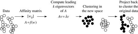
Figure 11.10 The framework of spectral clustering approaches. Source: Adapted from Slide 8 at http://videolectures.net/micued08_azran_mcl/.
Given a set of objects, ![]() , the distance between each pair of objects,
, the distance between each pair of objects, ![]()
![]() , and the desired number k of clusters, a spectral clustering approach works as follows.
, and the desired number k of clusters, a spectral clustering approach works as follows.
Using the distance measure, calculate an affinity matrix, W, such that
![]()
where σ is a scaling parameter that controls how fast the affinity Wij decreases as ![]() increases. In the Ng-Jordan-Weiss algorithm, Wii is set to 0.
increases. In the Ng-Jordan-Weiss algorithm, Wii is set to 0.
Using the affinity matrix W, derive a matrix ![]() . The way in which this is done can vary. The Ng-Jordan-Weiss algorithm defines a matrix, D, as a diagonal matrix such that Dii is the sum of the i th row of W, that is,
. The way in which this is done can vary. The Ng-Jordan-Weiss algorithm defines a matrix, D, as a diagonal matrix such that Dii is the sum of the i th row of W, that is,
![]() (11.24)
(11.24)
A is then set to
![]() (11.25)
(11.25)
Find the k leading eigenvectors of A. Recall that the eigenvectors of a square matrix are the nonzero vectors that remain proportional to the original vector after being multiplied by the matrix. Mathematically, a vector v is an eigenvector of matrix A if ![]() , where λ is called the corresponding eigenvalue. This step derives k new dimensions from A, which are based on the affinity matrix W. Typically, k should be much smaller than the dimensionality of the original data.
, where λ is called the corresponding eigenvalue. This step derives k new dimensions from A, which are based on the affinity matrix W. Typically, k should be much smaller than the dimensionality of the original data.
The Ng-Jordan-Weiss algorithm computes the k eigenvectors with the largest eigenvalues ![]() of A.
of A.
Using the k leading eigenvectors, project the original data into the new space defined by the k leading eigenvectors, and run a clustering algorithm such as k-means to find k clusters.
The Ng-Jordan-Weiss algorithm stacks the k largest eigenvectors in columns to form a matrix ![]() . The algorithm forms a matrix Y by renormalizing each row in X to have unit length, that is,
. The algorithm forms a matrix Y by renormalizing each row in X to have unit length, that is,
![]() (11.26)
(11.26)
The algorithm then treats each row in Y as a point in the k-dimensional space ![]() , and runs k-means (or any other algorithm serving the partitioning purpose) to cluster the points into k clusters.
, and runs k-means (or any other algorithm serving the partitioning purpose) to cluster the points into k clusters.
Assign the original data points to clusters according to how the transformed points are assigned in the clusters obtained in step 4.
In the Ng-Jordan-Weiss algorithm, the original object oi is assigned to the j th cluster if and only if matrix Y's row i is assigned to the j th cluster as a result of step 4.
In spectral clustering methods, the dimensionality of the new space is set to the desired number of clusters. This setting expects that each new dimension should be able to manifest a cluster.
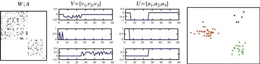
Figure 11.11 The new dimensions and the clustering results of the Ng-Jordan-Weiss algorithm. Source: Adapted from Slide 9 at http://videolectures.net/micued08_azran_mcl/.
Spectral clustering is effective in high-dimensional applications such as image processing. Theoretically, it works well when certain conditions apply. Scalability, however, is a challenge. Computing eigenvectors on a large matrix is costly. Spectral clustering can be combined with other clustering methods, such as biclustering. Additional information on other dimensionality reduction clustering methods, such as kernel PCA, can be found in the bibliographic notes (Section 11.7).