
11.1 Probabilistic Model-Based Clustering
In all the cluster analysis methods we have discussed so far, each data object can be assigned to only one of a number of clusters. This cluster assignment rule is required in some applications such as assigning customers to marketing managers. However, in other applications, this rigid requirement may not be desirable. In this section, we demonstrate the need for fuzzy or flexible cluster assignment in some applications, and introduce a general method to compute probabilistic clusters and assignments.
“In what situations may a data object belong to more than one cluster?” Consider Example 11.1.
The scenario where an object may belong to multiple clusters occurs often in many applications. This is illustrated in Example 11.2.
In this section, we systematically study the theme of clustering that allows an object to belong to more than one cluster. We start with the notion of fuzzy clusters in Section 11.1.1. We then generalize the concept to probabilistic model-based clusters in Section 11.1.2. In Section 11.1.3, we introduce the expectation-maximization algorithm, a general framework for mining such clusters.
11.1.1 Fuzzy Clusters
Given a set of objects, ![]() , a fuzzy set S is a subset of X that allows each object in X to have a membership degree between 0 and 1. Formally, a fuzzy set, S, can be modeled as a function,
, a fuzzy set S is a subset of X that allows each object in X to have a membership degree between 0 and 1. Formally, a fuzzy set, S, can be modeled as a function, ![]() .
.
Example 11.3
Fuzzy set
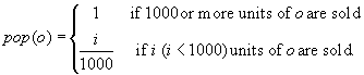
The more digital camera units that are sold, the more popular the camera is. In AllElectronics, we can use the following formula to compute the degree of popularity of a digital camera, o, given the sales of o:
 (11.1)
Function pop() defines a fuzzy set of popular digital cameras. For example, suppose the sales of digital cameras at AllElectronics are as shown in Table 11.1. The fuzzy set of popular digital cameras is ![]() , where the degrees of membership are written in parentheses.
, where the degrees of membership are written in parentheses.
Table 11.1
Set of Digital Cameras and Their Sales at AllElectronics
| Camera | Sales (units) |
| A | 50 |
| B | 1320 |
| C | 860 |
| D | 270 |
We can apply the fuzzy set idea on clusters. That is, given a set of objects, a cluster is a fuzzy set of objects. Such a cluster is called a fuzzy cluster. Consequently, a clustering contains multiple fuzzy clusters.
Formally, given a set of objects, o1, …, on, a fuzzy clustering of kfuzzy clusters, C1, …, Ck, can be represented using a partition matrix, ![]()
![]() , where wij is the membership degree of oi in fuzzy cluster Cj. The partition matrix should satisfy the following three requirements:
, where wij is the membership degree of oi in fuzzy cluster Cj. The partition matrix should satisfy the following three requirements:
■ For each object, oi, and cluster, Cj, ![]() . This requirement enforces that a fuzzy cluster is a fuzzy set.
. This requirement enforces that a fuzzy cluster is a fuzzy set.
■ For each object, oi, ![]() . This requirement ensures that every object participates in the clustering equivalently.
. This requirement ensures that every object participates in the clustering equivalently.
■ For each cluster, Cj, ![]() . This requirement ensures that for every cluster, there is at least one object for which the membership value is nonzero.
. This requirement ensures that for every cluster, there is at least one object for which the membership value is nonzero.
Example 11.4
Fuzzy clusters
Suppose the AllElectronics online store has six reviews. The keywords contained in these reviews are listed in Table 11.2.
We can group the reviews into two fuzzy clusters, C1 and C2. C1 is for “digital camera” and “lens," and C2 is for “computer.” The partition matrix is
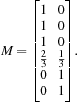
Here, we use the keywords “digital camera” and “lens” as the features of cluster C1, and “computer” as the feature of cluster C2. For review, Ri, and cluster, Cj![]() , wij is defined as
, wij is defined as
![]()
In this fuzzy clustering, review R4 belongs to clusters C1 and C2 with membership degrees ![]() and
and ![]() , respectively.
, respectively.
Table 11.2
Set of Reviews and the Keywords Used
| Review_ID | Keywords |
| R1 | digital camera, lens |
| R2 | digital camera |
| R3 | lens |
| R4 | digital camera, lens, computer |
| R5 | computer, CPU |
| R6 | computer, computer game |
“How can we evaluate how well a fuzzy clustering describes a data set?” Consider a set of objects, ![]() , and a fuzzy clustering
, and a fuzzy clustering ![]() of k clusters,
of k clusters, ![]() . Let
. Let ![]()
![]() be the partition matrix. Let
be the partition matrix. Let ![]() be the centers of clusters
be the centers of clusters ![]() , respectively. Here, a center can be defined either as the mean or the medoid, or in other ways specific to the application.
, respectively. Here, a center can be defined either as the mean or the medoid, or in other ways specific to the application.
As discussed in Chapter 10, the distance or similarity between an object and the center of the cluster to which the object is assigned can be used to measure how well the object belongs to the cluster. This idea can be extended to fuzzy clustering. For any object, oi, and cluster, Cj, if ![]() , then
, then ![]() measures how well oi is represented by cj, and thus belongs to cluster Cj. Because an object can participate in more than one cluster, the sum of distances to the corresponding cluster centers weighted by the degrees of membership captures how well the object fits the clustering.
measures how well oi is represented by cj, and thus belongs to cluster Cj. Because an object can participate in more than one cluster, the sum of distances to the corresponding cluster centers weighted by the degrees of membership captures how well the object fits the clustering.
Formally, for an object oi, the sum of the squared error (SSE) is given by
![]() (11.2)
(11.2)
where the parameter ![]() controls the influence of the degrees of membership. The larger the value of p, the larger the influence of the degrees of membership. Orthogonally, the SSE for a cluster, Cj, is
controls the influence of the degrees of membership. The larger the value of p, the larger the influence of the degrees of membership. Orthogonally, the SSE for a cluster, Cj, is
![]() (11.3)
(11.3)
Finally, the SSE of the clustering is defined as
![]() (11.4)
(11.4)
The SSE can be used to measure how well a fuzzy clustering fits a data set.
Fuzzy clustering is also called soft clustering because it allows an object to belong to more than one cluster. It is easy to see that traditional (rigid) clustering, which enforces each object to belong to only one cluster exclusively, is a special case of fuzzy clustering. We defer the discussion of how to compute fuzzy clustering to Section 11.1.3.
11.1.2 Probabilistic Model-Based Clusters
“Fuzzy clusters (Section 11.1.1) provide the flexibility of allowing an object to participate in multiple clusters. Is there a general framework to specify clusterings where objects may participate in multiple clusters in a probabilistic way?” In this section, we introduce the general notion of probabilistic model-based clusters to answer this question.
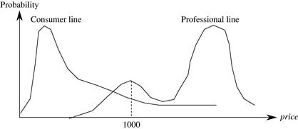
As discussed in Chapter 10, we conduct cluster analysis on a data set because we assume that the objects in the data set in fact belong to different inherent categories. Recall that clustering tendency analysis (Section 10.6.1) can be used to examine whether a data set contains objects that may lead to meaningful clusters. Here, the inherent categories hidden in the data are latent, which means they cannot be directly observed. Instead, we have to infer them using the data observed. For example, the topics hidden in a set of reviews in the AllElectronics online store are latent because one cannot read the topics directly. However, the topics can be inferred from the reviews because each review is about one or multiple topics.
Therefore, the goal of cluster analysis is to find hidden categories. A data set that is the subject of cluster analysis can be regarded as a sample of the possible instances of the hidden categories, but without any category labels. The clusters derived from cluster analysis are inferred using the data set, and are designed to approach the hidden categories.
Statistically, we can assume that a hidden category is a distribution over the data space, which can be mathematically represented using a probability density function (or distribution function). We call such a hidden category a probabilistic cluster. For a probabilistic cluster, C, its probability density function, f, and a point, o, in the data space, f(o) is the relative likelihood that an instance of C appears at o.
Suppose we want to find k probabilistic clusters, ![]() , through cluster analysis. For a data set, D, of n objects, we can regard D as a finite sample of the possible instances of the clusters. Conceptually, we can assume that D is formed as follows. Each cluster, Cj
, through cluster analysis. For a data set, D, of n objects, we can regard D as a finite sample of the possible instances of the clusters. Conceptually, we can assume that D is formed as follows. Each cluster, Cj![]() , is associated with a probability, ωj, that some instance is sampled from the cluster. It is often assumed that
, is associated with a probability, ωj, that some instance is sampled from the cluster. It is often assumed that ![]() are given as part of the problem setting, and that
are given as part of the problem setting, and that ![]() , which ensures that all objects are generated by the k clusters. Here, parameter ωj captures background knowledge about the relative population of cluster Cj.
, which ensures that all objects are generated by the k clusters. Here, parameter ωj captures background knowledge about the relative population of cluster Cj.
We then run the following two steps to generate an object in D. The steps are executed n times in total to generate n objects, ![]() , in D.
, in D.
1. Choose a cluster, Cj, according to probabilities ![]() .
.
2. Choose an instance of Cj according to its probability density function, fj.
The data generation process here is the basic assumption in mixture models. Formally, a mixture model assumes that a set of observed objects is a mixture of instances from multiple probabilistic clusters. Conceptually, each observed object is generated independently by two steps: first choosing a probabilistic cluster according to the probabilities of the clusters, and then choosing a sample according to the probability density function of the chosen cluster.
Given data set, D, and k, the number of clusters required, the task of probabilistic model-based cluster analysis is to infer a set of k probabilistic clusters that is most likely to generate D using this data generation process. An important question remaining is how we can measure the likelihood that a set of k probabilistic clusters and their probabilities will generate an observed data set.
Consider a set, C, of k probabilistic clusters, ![]() , with probability density functions
, with probability density functions ![]() , respectively, and their probabilities,
, respectively, and their probabilities, ![]() . For an object, o, the probability that o is generated by cluster Cj
. For an object, o, the probability that o is generated by cluster Cj![]() is given by
is given by ![]() . Therefore, the probability that o is generated by the set C of clusters is
. Therefore, the probability that o is generated by the set C of clusters is
![]() (11.5)
(11.5)
Since the objects are assumed to have been generated independently, for a data set, ![]() , of n objects, we have
, of n objects, we have
![]() (11.6)
(11.6)
Now, it is clear that the task of probabilistic model-based cluster analysis on a data set, D, is to find a set C of k probabilistic clusters such that ![]() is maximized. Maximizing
is maximized. Maximizing ![]() is often intractable because, in general, the probability density function of a cluster can take an arbitrarily complicated form. To make probabilistic model-based clusters computationally feasible, we often compromise by assuming that the probability density functions are parameterized distributions.
is often intractable because, in general, the probability density function of a cluster can take an arbitrarily complicated form. To make probabilistic model-based clusters computationally feasible, we often compromise by assuming that the probability density functions are parameterized distributions.
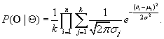
Formally, let ![]() be the n observed objects, and
be the n observed objects, and ![]() be the parameters of the k distributions, denoted by
be the parameters of the k distributions, denoted by ![]() and
and ![]() , respectively. Then, for any object,
, respectively. Then, for any object, ![]()
![]() , Eq. (11.5) can be rewritten as
, Eq. (11.5) can be rewritten as
![]() (11.7)
(11.7)
where ![]() is the probability that oi is generated from the j th distribution using parameter Θj. Consequently, Eq. (11.6) can be rewritten as
is the probability that oi is generated from the j th distribution using parameter Θj. Consequently, Eq. (11.6) can be rewritten as
![]() (11.8)
(11.8)
Using the parameterized probability distribution models, the task of probabilistic model-based cluster analysis is to infer a set of parameters, Θ, that maximizes Eq. (11.8).
Example 11.6
Univariate Gaussian mixture model
Let’s use univariate Gaussian distributions as an example. That is, we assume that the probability density function of each cluster follows a 1-D Gaussian distribution. Suppose there are k clusters. The two parameters for the probability density function of each cluster are center, μj, and standard deviation, σj![]() . We denote the parameters as
. We denote the parameters as ![]() and
and ![]() . Let the data set be
. Let the data set be ![]() , where oi
, where oi![]() is a real number. For any point,
is a real number. For any point, ![]() , we have
, we have
![]() (11.9)
(11.9)
Assuming that each cluster has the same probability, that is ![]() , and plugging Eq. (11.9) into Eq. (11.7), we have
, and plugging Eq. (11.9) into Eq. (11.7), we have
 (11.10)
Applying Eq. (11.8), we have
 (11.11)
The task of probabilistic model-based cluster analysis using a univariate Gaussian mixture model is to infer Θ such that Eq. (11.11) is maximized.
11.1.3 Expectation-Maximization Algorithm
“How can we compute fuzzy clusterings and probabilistic model-based clusterings?” In this section, we introduce a principled approach. Let’s start with a review of the k-means clustering problem and the k-means algorithm studied in Chapter 10.
It can easily be shown that k-means clustering is a special case of fuzzy clustering (Exercise 11.1). The k-means algorithm iterates until the clustering cannot be improved. Each iteration consists of two steps:
The expectation step (E-step): Given the current cluster centers, each object is assigned to the cluster with a center that is closest to the object. Here, an object is expected to belong to the closest cluster.
The maximization step (M-step): Given the cluster assignment, for each cluster, the algorithm adjusts the center so that the sum of the distances from the objects assigned to this cluster and the new center is minimized. That is, the similarity of objects assigned to a cluster is maximized.
We can generalize this two-step method to tackle fuzzy clustering and probabilistic model-based clustering. In general, an expectation-maximization (EM) algorithm is a framework that approaches maximum likelihood or maximum a posteriori estimates of parameters in statistical models. In the context of fuzzy or probabilistic model-based clustering, an EM algorithm starts with an initial set of parameters and iterates until the clustering cannot be improved, that is, until the clustering converges or the change is sufficiently small (less than a preset threshold). Each iteration also consists of two steps:
■ The expectation step assigns objects to clusters according to the current fuzzy clustering or parameters of probabilistic clusters.
■ The maximization step finds the new clustering or parameters than minimize the SSE in fuzzy clustering (Eq. 11.4) or the expected likelihood in probabilistic model-based clustering.
Example 11.7
Fuzzy clustering using the EM algorithm
Consider the six points in Figure 11.2, where the coordinates of the points are also shown. Let’s compute two fuzzy clusters using the EM algorithm.
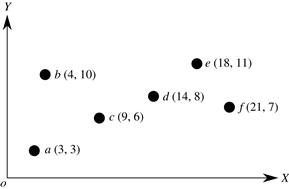
We randomly select two points, say ![]() and
and ![]() , as the initial centers of the two clusters. The first iteration conducts the expectation step and the maximization step as follows.
, as the initial centers of the two clusters. The first iteration conducts the expectation step and the maximization step as follows.
In the E-step, for each point we calculate its membership degree in each cluster. For any point, o, we assign o to c1 and c2 with membership weights
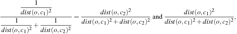
respectively, where ![]() is the Euclidean distance. The rationale is that, if o is close to c1 and
is the Euclidean distance. The rationale is that, if o is close to c1 and ![]() is small, the membership degree of o with respect to c1 should be high. We also normalize the membership degrees so that the sum of degrees for an object is equal to 1.
is small, the membership degree of o with respect to c1 should be high. We also normalize the membership degrees so that the sum of degrees for an object is equal to 1.
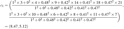
For point a, we have ![]() and
and ![]() . That is, a exclusively belongs to c1. For point b, we have
. That is, a exclusively belongs to c1. For point b, we have ![]() and
and ![]() . For point c, we have
. For point c, we have ![]() and
and ![]() . The degrees of membership of the other points are shown in the partition matrix in Table 11.3.
. The degrees of membership of the other points are shown in the partition matrix in Table 11.3.

In the M-step, we recalculate the centroids according to the partition matrix, minimizing the SSE given in Eq. (11.4). The new centroid should be adjusted to
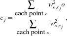 (11.12)
where ![]() .
.
and
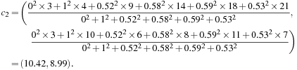
We repeat the iterations, where each iteration contains an E-step and an M-step. Table 11.3 shows the results from the first three iterations. The algorithm stops when the cluster centers converge or the change is small enough.
“How can we apply the EM algorithm to compute probabilistic model-based clustering?” Let’s use a univariate Gaussian mixture model (Example 11.6) to illustrate.
Example 11.8
Using the EM algorithm for mixture models
Given a set of objects, ![]() , we want to mine a set of parameters,
, we want to mine a set of parameters, ![]() , such that
, such that ![]() in Eq. (11.11) is maximized, where
in Eq. (11.11) is maximized, where ![]() are the mean and standard deviation, respectively, of the j th univariate Gaussian distribution,
are the mean and standard deviation, respectively, of the j th univariate Gaussian distribution, ![]() .
.
We can apply the EM algorithm. We assign random values to parameters Θ as the initial values. We then iteratively conduct the E-step and the M-step as follows until the parameters converge or the change is sufficiently small.
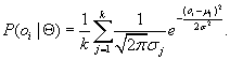
In the E-step, for each object, ![]()
![]() , we calculate the probability that oi belongs to each distribution, that is,
, we calculate the probability that oi belongs to each distribution, that is,
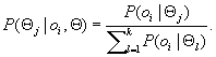 (11.13)
In the M-step, we adjust the parameters Θ so that the expected likelihood ![]() in Eq. (11.11) is maximized. This can be achieved by setting
in Eq. (11.11) is maximized. This can be achieved by setting
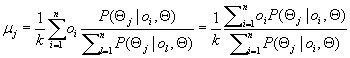 (11.14)
and
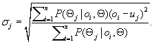 (11.15)
In many applications, probabilistic model-based clustering has been shown to be effective because it is more general than partitioning methods and fuzzy clustering methods. A distinct advantage is that appropriate statistical models can be used to capture latent clusters. The EM algorithm is commonly used to handle many learning problems in data mining and statistics due to its simplicity. Note that, in general, the EM algorithm may not converge to the optimal solution. It may instead converge to a local maximum. Many heuristics have been explored to avoid this. For example, we could run the EM process multiple times using different random initial values. Furthermore, the EM algorithm can be very costly if the number of distributions is large or the data set contains very few observed data points.