
9.1 Bayesian Belief Networks
Chapter 8 introduced Bayes' theorem and naïve Bayesian classification. In this chapter, we describe Bayesian belief networks —probabilistic graphical models, which unlike naïve Bayesian classifiers allow the representation of dependencies among subsets of attributes. Bayesian belief networks can be used for classification. Section 9.1.1 introduces the basic concepts of Bayesian belief networks. In Section 9.1.2, you will learn how to train such models.
9.1.1 Concepts and Mechanisms
The naïve Bayesian classifier makes the assumption of class conditional independence, that is, given the class label of a tuple, the values of the attributes are assumed to be conditionally independent of one another. This simplifies computation. When the assumption holds true, then the naïve Bayesian classifier is the most accurate in comparison with all other classifiers. In practice, however, dependencies can exist between variables. Bayesian belief networks specify joint conditional probability distributions. They allow class conditional independencies to be defined between subsets of variables. They provide a graphical model of causal relationships, on which learning can be performed. Trained Bayesian belief networks can be used for classification. Bayesian belief networks are also known as belief networks, Bayesian networks, and probabilistic networks. For brevity, we will refer to them as belief networks.
A belief network is defined by two components—a directed acyclic graph and a set of conditional probability tables (Figure 9.1). Each node in the directed acyclic graph represents a random variable. The variables may be discrete- or continuous-valued. They may correspond to actual attributes given in the data or to “hidden variables” believed to form a relationship (e.g., in the case of medical data, a hidden variable may indicate a syndrome, representing a number of symptoms that, together, characterize a specific disease). Each arc represents a probabilistic dependence. If an arc is drawn from a node Y to a node Z, then Y is a parent or immediate predecessor of Z, and Z is a descendant of Y. Each variable is conditionally independent of its nondescendants in the graph, given its parents.
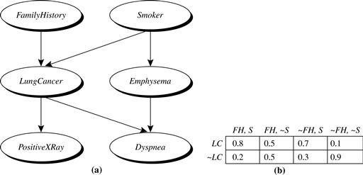
Figure 9.1 Simple Bayesian belief network. (a) A proposed causal model, represented by a directed acyclic graph. (b) The conditional probability table for the values of the variable LungCancer (LC) showing each possible combination of the values of its parent nodes, FamilyHistory (FH) and Smoker (S). Source: Adapted from Russell, Binder, Koller, and Kanazawa [RBKK95].
Figure 9.1 is a simple belief network, adapted from Russell, Binder, Koller, and Kanazawa [RBKK95] for six Boolean variables. The arcs in Figure 9.1(a) allow a representation of causal knowledge. For example, having lung cancer is influenced by a person’s family history of lung cancer, as well as whether or not the person is a smoker. Note that the variable PositiveXRay is independent of whether the patient has a family history of lung cancer or is a smoker, given that we know the patient has lung cancer. In other words, once we know the outcome of the variable LungCancer, then the variables FamilyHistory and Smoker do not provide any additional information regarding PositiveXRay. The arcs also show that the variable LungCancer is conditionally independent of Emphysema, given its parents, FamilyHistory and Smoker.
A belief network has one conditional probability table (CPT) for each variable. The CPT for a variable Y specifies the conditional distribution ![]() , where
, where ![]() are the parents of Y. Figure 9.1(b) shows a CPT for the variable LungCancer. The conditional probability for each known value of LungCancer is given for each possible combination of the values of its parents. For instance, from the upper leftmost and bottom rightmost entries, respectively, we see that
are the parents of Y. Figure 9.1(b) shows a CPT for the variable LungCancer. The conditional probability for each known value of LungCancer is given for each possible combination of the values of its parents. For instance, from the upper leftmost and bottom rightmost entries, respectively, we see that
![]()
Let ![]() be a data tuple described by the variables or attributes
be a data tuple described by the variables or attributes ![]() , respectively. Recall that each variable is conditionally independent of its nondescendants in the network graph, given its parents. This allows the network to provide a complete representation of the existing joint probability distribution with the following equation:
, respectively. Recall that each variable is conditionally independent of its nondescendants in the network graph, given its parents. This allows the network to provide a complete representation of the existing joint probability distribution with the following equation:
![]() (9.1)
(9.1)
where ![]() is the probability of a particular combination of values of X, and the values for
is the probability of a particular combination of values of X, and the values for ![]() correspond to the entries in the CPT for Yi.
correspond to the entries in the CPT for Yi.
A node within the network can be selected as an “output” node, representing a class label attribute. There may be more than one output node. Various algorithms for inference and learning can be applied to the network. Rather than returning a single class label, the classification process can return a probability distribution that gives the probability of each class. Belief networks can be used to answer probability of evidence queries (e.g., what is the probability that an individual will have LungCancer, given that they have both PositiveXRay and Dyspnea) and most probable explanation queries (e.g., which group of the population is most likely to have both PositiveXRay and Dyspnea).
Belief networks have been used to model a number of well-known problems. One example is genetic linkage analysis (e.g., the mapping of genes onto a chromosome). By casting the gene linkage problem in terms of inference on Bayesian networks, and using state-of-the art algorithms, the scalability of such analysis has advanced considerably. Other applications that have benefited from the use of belief networks include computer vision (e.g., image restoration and stereo vision), document and text analysis, decision-support systems, and sensitivity analysis. The ease with which many applications can be reduced to Bayesian network inference is advantageous in that it curbs the need to invent specialized algorithms for each such application.
9.1.2 Training Bayesian Belief Networks
“How does a Bayesian belief network learn?” In the learning or training of a belief network, a number of scenarios are possible. The network topology (or “layout” of nodes and arcs) may be constructed by human experts or inferred from the data. The network variables may be observable or hidden in all or some of the training tuples. The hidden data case is also referred to as missing values or incomplete data.
Several algorithms exist for learning the network topology from the training data given observable variables. The problem is one of discrete optimization. For solutions, please see the bibliographic notes at the end of this chapter (Section 9.10). Human experts usually have a good grasp of the direct conditional dependencies that hold in the domain under analysis, which helps in network design. Experts must specify conditional probabilities for the nodes that participate in direct dependencies. These probabilities can then be used to compute the remaining probability values.
If the network topology is known and the variables are observable, then training the network is straightforward. It consists of computing the CPT entries, as is similarly done when computing the probabilities involved in naïve Bayesian classification.
When the network topology is given and some of the variables are hidden, there are various methods to choose from for training the belief network. We will describe a promising method of gradient descent. For those without an advanced math background, the description may look rather intimidating with its calculus-packed formulae. However, packaged software exists to solve these equations, and the general idea is easy to follow.
Let D be a training set of data tuples, ![]() . Training the belief network means that we must learn the values of the CPT entries. Let
. Training the belief network means that we must learn the values of the CPT entries. Let ![]() be a CPT entry for the variable
be a CPT entry for the variable ![]() having the parents
having the parents ![]() , where
, where ![]() . For example, if
. For example, if ![]() is the upper leftmost CPT entry of Figure 9.1(b), then Yi is LungCancer;
is the upper leftmost CPT entry of Figure 9.1(b), then Yi is LungCancer; ![]() is its value,” yes ”; Ui lists the parent nodes of Yi, namely, {FamilyHistory, Smoker}; and
is its value,” yes ”; Ui lists the parent nodes of Yi, namely, {FamilyHistory, Smoker}; and ![]() lists the values of the parent nodes, namely, { “yes”, “yes”}. The
lists the values of the parent nodes, namely, { “yes”, “yes”}. The ![]() are viewed as weights, analogous to the weights in hidden units of neural networks (Section 9.2). The set of weights is collectively referred to as W. The weights are initialized to random probability values. A gradient descent strategy performs greedy hill-climbing. At each iteration, the weights are updated and will eventually converge to a local optimum solution.
are viewed as weights, analogous to the weights in hidden units of neural networks (Section 9.2). The set of weights is collectively referred to as W. The weights are initialized to random probability values. A gradient descent strategy performs greedy hill-climbing. At each iteration, the weights are updated and will eventually converge to a local optimum solution.
A gradient descent strategy is used to search for the ![]() values that best model the data, based on the assumption that each possible setting of
values that best model the data, based on the assumption that each possible setting of ![]() is equally likely. Such a strategy is iterative. It searches for a solution along the negative of the gradient (i.e., steepest descent) of a criterion function. We want to find the set of weights, W, that maximize this function. To start with, the weights are initialized to random probability values. The gradient descent method performs greedy hill-climbing in that, at each iteration or step along the way, the algorithm moves toward what appears to be the best solution at the moment, without backtracking. The weights are updated at each iteration. Eventually, they converge to a local optimum solution.
is equally likely. Such a strategy is iterative. It searches for a solution along the negative of the gradient (i.e., steepest descent) of a criterion function. We want to find the set of weights, W, that maximize this function. To start with, the weights are initialized to random probability values. The gradient descent method performs greedy hill-climbing in that, at each iteration or step along the way, the algorithm moves toward what appears to be the best solution at the moment, without backtracking. The weights are updated at each iteration. Eventually, they converge to a local optimum solution.
For our problem, we maximize ![]() . This can be done by following the gradient of
. This can be done by following the gradient of ![]() , which makes the problem simpler. Given the network topology and initialized
, which makes the problem simpler. Given the network topology and initialized ![]() , the algorithm proceeds as follows:
, the algorithm proceeds as follows:
1. Compute the gradients: For each i, j, k, compute
![]() (9.2)
(9.2)
The probability on the right side of Eq. (9.2) is to be calculated for each training tuple, ![]() , in D. For brevity, let’s refer to this probability simply as p. When the variables represented by Yi and Ui are hidden for some
, in D. For brevity, let’s refer to this probability simply as p. When the variables represented by Yi and Ui are hidden for some ![]() , then the corresponding probability p can be computed from the observed variables of the tuple using standard algorithms for Bayesian network inference such as those available in the commercial software package HUGIN (www.hugin.dk).
, then the corresponding probability p can be computed from the observed variables of the tuple using standard algorithms for Bayesian network inference such as those available in the commercial software package HUGIN (www.hugin.dk).
2. Take a small step in the direction of the gradient: The weights are updated by
![]() (9.3)
(9.3)
where l is the learning rate representing the step size and ![]() is computed from Eq. (9.2). The learning rate is set to a small constant and helps with convergence.
is computed from Eq. (9.2). The learning rate is set to a small constant and helps with convergence.
Renormalize the weights: Because the weights ![]() are probability values, they must be between 0.0 and 1.0, and
are probability values, they must be between 0.0 and 1.0, and ![]() must equal 1 for all i, k. These criteria are achieved by renormalizing the weights after they have been updated by Eq. (9.3).
must equal 1 for all i, k. These criteria are achieved by renormalizing the weights after they have been updated by Eq. (9.3).
Algorithms that follow this learning form are called adaptive probabilistic networks. Other methods for training belief networks are referenced in the bibliographic notes at the end of this chapter (Section 9.10). Belief networks are computationally intensive. Because belief networks provide explicit representations of causal structure, a human expert can provide prior knowledge to the training process in the form of network topology and/or conditional probability values. This can significantly improve the learning rate.