
5.1 Data Cube Computation: Preliminary Concepts
Data cubes facilitate the online analytical processing of multidimensional data. “But how can we compute data cubes in advance, so that they are handy and readily available for query processing?” This section contrasts full cube materialization (i.e., precomputation) versus various strategies for partial cube materialization. For completeness, we begin with a review of the basic terminology involving data cubes. We also introduce a cube cell notation that is useful for describing data cube computation methods.
5.1.1 Cube Materialization: Full Cube, Iceberg Cube, Closed Cube, and Cube Shell
Figure 5.1 shows a 3-D data cube for the dimensions A, B, and C, and an aggregate measure, M. Commonly used measures include count(), sum(), min(), max(), and total_sales(). A data cube is a lattice of cuboids. Each cuboid represents a group-by. ABC is the base cuboid, containing all three of the dimensions. Here, the aggregate measure, M, is computed for each possible combination of the three dimensions. The base cuboid is the least generalized of all the cuboids in the data cube. The most generalized cuboid is the apex cuboid, commonly represented as all. It contains one value—it aggregates measure M for all the tuples stored in the base cuboid. To drill down in the data cube, we move from the apex cuboid downward in the lattice. To roll up, we move from the base cuboid upward. For the purposes of our discussion in this chapter, we will always use the term data cube to refer to a lattice of cuboids rather than an individual cuboid.
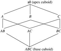
Figure 5.1 Lattice of cuboids making up a 3-D data cube with the dimensions A, B, and C for some aggregate measure, M.
A cell in the base cuboid is a base cell. A cell from a nonbase cuboid is an aggregate cell. An aggregate cell aggregates over one or more dimensions, where each aggregated dimension is indicated by a ∗ in the cell notation. Suppose we have an n-dimensional data cube. Let a = (a1, a2, …, an, measures) be a cell from one of the cuboids making up the data cube. We say that a is an m-dimensional cell (i.e., from an m-dimensional cuboid) if exactly m (m ≤ n) values among {a1, a2, …, an} are not ∗. If m = n, then a is a base cell; otherwise, it is an aggregate cell (i.e., where m < n).
An ancestor–descendant relationship may exist between cells. In an n-dimensional data cube, an i-D cell a = (a1, a2, …, an, measuresa) is an ancestor of a j-D cell b = (b1, b2, …, bn, measuresb), and b is a descendant of a, if and only if (1) i < j, and (2) for 1 ≤ k ≤ n, ak = bk whenever ak ≠ ∗. In particular, cell a is called a parent of cell b, and b is a child of a, if and only if j = i + 1.
To ensure fast OLAP, it is sometimes desirable to precompute the full cube (i.e., all the cells of all the cuboids for a given data cube). A method of full cube computation is given in Section 5.2.1. Full cube computation, however, is exponential to the number of dimensions. That is, a data cube of n dimensions contains 2n cuboids. There are even more cuboids if we consider concept hierarchies for each dimension.1 In addition, the size of each cuboid depends on the cardinality of its dimensions. Thus, precomputation of the full cube can require huge and often excessive amounts of memory.
Nonetheless, full cube computation algorithms are important. Individual cuboids may be stored on secondary storage and accessed when necessary. Alternatively, we can use such algorithms to compute smaller cubes, consisting of a subset of the given set of dimensions, or a smaller range of possible values for some of the dimensions. In these cases, the smaller cube is a full cube for the given subset of dimensions and/or dimension values. A thorough understanding of full cube computation methods will help us develop efficient methods for computing partial cubes. Hence, it is important to explore scalable methods for computing all the cuboids making up a data cube, that is, for full materialization. These methods must take into consideration the limited amount of main memory available for cuboid computation, the total size of the computed data cube, as well as the time required for such computation.
Partial materialization of data cubes offers an interesting trade-off between storage space and response time for OLAP. Instead of computing the full cube, we can compute only a subset of the data cube’s cuboids, or subcubes consisting of subsets of cells from the various cuboids.
Many cells in a cuboid may actually be of little or no interest to the data analyst. Recall that each cell in a full cube records an aggregate value such as count or sum. For many cells in a cuboid, the measure value will be zero. When the product of the cardinalities for the dimensions in a cuboid is large relative to the number of nonzero-valued tuples that are stored in the cuboid, then we say that the cuboid is sparse. If a cube contains many sparse cuboids, we say that the cube is sparse.
In many cases, a substantial amount of the cube’s space could be taken up by a large number of cells with very low measure values. This is because the cube cells are often quite sparsely distributed within a multidimensional space. For example, a customer may only buy a few items in a store at a time. Such an event will generate only a few nonempty cells, leaving most other cube cells empty. In such situations, it is useful to materialize only those cells in a cuboid (group-by) with a measure value above some minimum threshold. In a data cube for sales, say, we may wish to materialize only those cells for which count ≥ 10 (i.e., where at least 10 tuples exist for the cell’s given combination of dimensions), or only those cells representing sales ≥ $100. This not only saves processing time and disk space, but also leads to a more focused analysis. The cells that cannot pass the threshold are likely to be too trivial to warrant further analysis.
Such partially materialized cubes are known as iceberg cubes. The minimum threshold is called the minimum support threshold, or minimum support (min_sup), for short. By materializing only a fraction of the cells in a data cube, the result is seen as the “tip of the iceberg,” where the “iceberg” is the potential full cube including all cells. An iceberg cube can be specified with an SQL query, as shown in Example 5.3.
A naïve approach to computing an iceberg cube would be to first compute the full cube and then prune the cells that do not satisfy the iceberg condition. However, this is still prohibitively expensive. An efficient approach is to compute only the iceberg cube directly without computing the full cube. Sections 5.2.2 and 5.2.3 discuss methods for efficient iceberg cube computation.
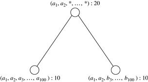
Introducing iceberg cubes will lessen the burden of computing trivial aggregate cells in a data cube. However, we could still end up with a large number of uninteresting cells to compute. For example, suppose that there are 2 base cells for a database of 100 dimensions, denoted as {(a1, a2, a3, …, a100) : 10, (a1, a2, b3, …, b100) : 10}, where each has a cell count of 10. If the minimum support is set to 10, there will still be an impermissible number of cells to compute and store, although most of them are not interesting. For example, there are 2101 − 6 distinct aggregate cells,2 like {(a1, a2, a3, a4, …, a99, ∗) : 10, …, (a1, a2, ∗, a4, …, a99, a100) : 10, …, (a1, a2, a3, ∗, …, ∗, ∗) : 10}, but most of them do not contain much new information. If we ignore all the aggregate cells that can be obtained by replacing some constants by ∗’s while keeping the same measure value, there are only three distinct cells left: {(a1, a2, a3, …, a100) : 10, (a1, a2, b3, …, b100) : 10, (a1, a2, ∗, …, ∗) : 20}. That is, out of 2101 − 4 distinct base and aggregate cells, only three really offer valuable information.
To systematically compress a data cube, we need to introduce the concept of closed coverage. A cell, c, is a closed cell if there exists no cell, d, such that d is a specialization (descendant) of cell c (i.e., where d is obtained by replacing ∗ in c with a non-∗ value), and d has the same measure value as c. A closed cube is a data cube consisting of only closed cells. For example, the three cells derived in the preceding paragraph are the three closed cells of the data cube for the data set {(a1, a2, a3, …, a100) : 10, (a1, a2, b3, …, b100) : 10}. They form the lattice of a closed cube as shown in Figure 5.2. Other nonclosed cells can be derived from their corresponding closed cells in this lattice. For example, “(a1, ∗, ∗, …, ∗) : 20” can be derived from “(a1, a2, ∗, …, ∗) : 20” because the former is a generalized nonclosed cell of the latter. Similarly, we have “(a1, a2, b3, ∗, …, ∗) : 10.”
Another strategy for partial materialization is to precompute only the cuboids involving a small number of dimensions such as three to five. These cuboids form a cube shell for the corresponding data cube. Queries on additional combinations of the dimensions will have to be computed on-the-fly. For example, we could compute all cuboids with three dimensions or less in an n-dimensional data cube, resulting in a cube shell of size 3. This, however, can still result in a large number of cuboids to compute, particularly when n is large. Alternatively, we can choose to precompute only portions or fragments of the cube shell based on cuboids of interest. Section 5.2.4 discusses a method for computing shell fragments and explores how they can be used for efficient OLAP query processing.
5.1.2 General Strategies for Data Cube Computation
There are several methods for efficient data cube computation, based on the various kinds of cubes described in Section 5.1.1. In general, there are two basic data structures used for storing cuboids. The implementation of relational OLAP (ROLAP) uses relational tables, whereas multidimensional arrays are used in multidimensional OLAP (MOLAP). Although ROLAP and MOLAP may each explore different cube computation techniques, some optimization “tricks” can be shared among the different data representations. The following are general optimization techniques for efficient computation of data cubes.
Optimization Technique 1: Sorting, hashing, and grouping. Sorting, hashing, and grouping operations should be applied to the dimension attributes to reorder and cluster related tuples.
In cube computation, aggregation is performed on the tuples (or cells) that share the same set of dimension values. Thus, it is important to explore sorting, hashing, and grouping operations to access and group such data together to facilitate computation of such aggregates.
To compute total sales by branch, day, and item, for example, it can be more efficient to sort tuples or cells by branch, and then by day, and then group them according to the item name. Efficient implementations of such operations in large data sets have been extensively studied in the database research community. Such implementations can be extended to data cube computation.
This technique can also be further extended to perform shared-sorts (i.e., sharing sorting costs across multiple cuboids when sort-based methods are used), or to perform shared-partitions (i.e., sharing the partitioning cost across multiple cuboids when hash-based algorithms are used).
Optimization Technique 2: Simultaneous aggregation and caching of intermediate results. In cube computation, it is efficient to compute higher-level aggregates from previously computed lower-level aggregates, rather than from the base fact table. Moreover, simultaneous aggregation from cached intermediate computation results may lead to the reduction of expensive disk input/output (I/O) operations.
To compute sales by branch, for example, we can use the intermediate results derived from the computation of a lower-level cuboid such as sales by branch and day. This technique can be further extended to perform amortized scans (i.e., computing as many cuboids as possible at the same time to amortize disk reads).
Optimization Technique 3: Aggregation from the smallest child when there exist multiple child cuboids. When there exist multiple child cuboids, it is usually more efficient to compute the desired parent (i.e., more generalized) cuboid from the smallest, previously computed child cuboid.
To compute a sales cuboid, Cbranch, when there exist two previously computed cuboids, C{branch, year} and C{branch, item}, for example, it is obviously more efficient to compute Cbranch from the former than from the latter if there are many more distinct items than distinct years.
Many other optimization techniques may further improve computational efficiency. For example, string dimension attributes can be mapped to integers with values ranging from zero to the cardinality of the attribute.
In iceberg cube computation the following optimization technique plays a particularly important role.
Optimization Technique 4: The Apriori pruning method can be explored to compute iceberg cubes efficiently. The Apriori property,3 in the context of data cubes, states as follows: If a given cell does not satisfy minimum support, then no descendant of the cell (i.e., more specialized cell) will satisfy minimum support either. This property can be used to substantially reduce the computation of iceberg cubes.
Recall that the specification of iceberg cubes contains an iceberg condition, which is a constraint on the cells to be materialized. A common iceberg condition is that the cells must satisfy a minimum support threshold such as a minimum count or sum. In this situation, the Apriori property can be used to prune away the exploration of the cell’s descendants. For example, if the count of a cell, c, in a cuboid is less than a minimum support threshold, v, then the count of any of c’s descendant cells in the lower-level cuboids can never be greater than or equal to v, and thus can be pruned.
In other words, if a condition (e.g., the iceberg condition specified in the having clause) is violated for some cell c, then every descendant of c will also violate that condition. Measures that obey this property are known as antimonotonic.4 This form of pruning was made popular in frequent pattern mining, yet also aids in data cube computation by cutting processing time and disk space requirements. It can lead to a more focused analysis because cells that cannot pass the threshold are unlikely to be of interest.
In the following sections, we introduce several popular methods for efficient cube computation that explore these optimization strategies.