
6.2 Frequent Itemset Mining Methods
In this section, you will learn methods for mining the simplest form of frequent patterns such as those discussed for market basket analysis in Section 6.1.1. We begin by presenting Apriori, the basic algorithm for finding frequent itemsets (Section 6.2.1). In Section 6.2.2, we look at how to generate strong association rules from frequent itemsets. Section 6.2.3 describes several variations to the Apriori algorithm for improved efficiency and scalability. Section 6.2.4 presents pattern-growth methods for mining frequent itemsets that confine the subsequent search space to only the data sets containing the current frequent itemsets. Section 6.2.5 presents methods for mining frequent itemsets that take advantage of the vertical data format.
6.2.1 Apriori Algorithm: Finding Frequent Itemsets by Confined Candidate Generation
Apriori is a seminal algorithm proposed by R. Agrawal and R. Srikant in 1994 for mining frequent itemsets for Boolean association rules [AS94b]. The name of the algorithm is based on the fact that the algorithm uses prior knowledge of frequent itemset properties, as we shall see later. Apriori employs an iterative approach known as a level-wise search, where k-itemsets are used to explore (k + 1)-itemsets. First, the set of frequent 1-itemsets is found by scanning the database to accumulate the count for each item, and collecting those items that satisfy minimum support. The resulting set is denoted by L1. Next, L1 is used to find L2, the set of frequent 2-itemsets, which is used to find L3, and so on, until no more frequent k-itemsets can be found. The finding of each Lk requires one full scan of the database.
To improve the efficiency of the level-wise generation of frequent itemsets, an important property called the Apriori property is used to reduce the search space.
Apriori property: All nonempty subsets of a frequent itemset must also be frequent.
The Apriori property is based on the following observation. By definition, if an itemset I does not satisfy the minimum support threshold, min_sup, then I is not frequent, that is, ![]() . If an item A is added to the itemset I, then the resulting itemset (i.e.,
. If an item A is added to the itemset I, then the resulting itemset (i.e., ![]() ) cannot occur more frequently than I. Therefore,
) cannot occur more frequently than I. Therefore, ![]() is not frequent either, that is,
is not frequent either, that is, ![]() .
.
This property belongs to a special category of properties called antimonotonicity in the sense that if a set cannot pass a test, all of its supersets will fail the same test as well. It is called antimonotonicity because the property is monotonic in the context of failing a test.6
“How is the Apriori property used in the algorithm?” To understand this, let us look at how Lk − 1 is used to find Lk for ![]() . A two-step process is followed, consisting of join and prune actions.
. A two-step process is followed, consisting of join and prune actions.
1. The join step: To find Lk, a set of candidate k-itemsets is generated by joining Lk − 1 with itself. This set of candidates is denoted Ck. Let l1 and l2 be itemsets in Lk − 1. The notation ![]() refers to the j th item in li (e.g.,
refers to the j th item in li (e.g., ![]() refers to the second to the last item in l1). For efficient implementation, Apriori assumes that items within a transaction or itemset are sorted in lexicographic order. For the (k − 1)-itemset, li, this means that the items are sorted such that
refers to the second to the last item in l1). For efficient implementation, Apriori assumes that items within a transaction or itemset are sorted in lexicographic order. For the (k − 1)-itemset, li, this means that the items are sorted such that ![]() . The join,
. The join, ![]() , is performed, where members of Lk − 1 are joinable if their first
, is performed, where members of Lk − 1 are joinable if their first ![]() items are in common. That is, members l1 and l2 of Lk − 1 are joined if (
items are in common. That is, members l1 and l2 of Lk − 1 are joined if (![]()
![]() . The condition
. The condition ![]() simply ensures that no duplicates are generated. The resulting itemset formed by joining l1 and l2 is
simply ensures that no duplicates are generated. The resulting itemset formed by joining l1 and l2 is ![]() .
.
2. The prune step: Ck is a superset of Lk, that is, its members may or may not be frequent, but all of the frequent k-itemsets are included in Ck. A database scan to determine the count of each candidate in Ck would result in the determination of Lk (i.e., all candidates having a count no less than the minimum support count are frequent by definition, and therefore belong to Lk). Ck, however, can be huge, and so this could involve heavy computation. To reduce the size of Ck, the Apriori property is used as follows. Any (k − 1)-itemset that is not frequent cannot be a subset of a frequent k-itemset. Hence, if any (k − 1)-subset of a candidate k-itemset is not in Lk − 1, then the candidate cannot be frequent either and so can be removed from Ck. This subset testing can be done quickly by maintaining a hash tree of all frequent itemsets.
Example 6.3
Apriori
Let’s look at a concrete example, based on the AllElectronics transaction database, D, of Table 6.1. There are nine transactions in this database, that is, ![]() . We use Figure 6.2 to illustrate the Apriori algorithm for finding frequent itemsets in D.
. We use Figure 6.2 to illustrate the Apriori algorithm for finding frequent itemsets in D.
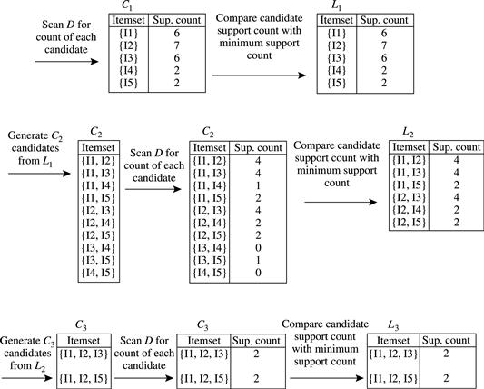
Figure 6.2 Generation of the candidate itemsets and frequent itemsets, where the minimum support count is 2.
Table 6.1
Transactional Data for an AllElectronics Branch
| TID | List of item_IDs |
| T100 | I1, I2, I5 |
| T200 | I2, I4 |
| T300 | I2, I3 |
| T400 | I1, I2, I4 |
| T500 | I1, I3 |
| T600 | I2, I3 |
| T700 | I1, I3 |
| T800 | I1, I2, I3, I5 |
| T900 | I1, I2, I3 |
1. In the first iteration of the algorithm, each item is a member of the set of candidate 1-itemsets, C1. The algorithm simply scans all of the transactions to count the number of occurrences of each item.
2. Suppose that the minimum support count required is 2, that is, ![]() . (Here, we are referring to absolute support because we are using a support count. The corresponding relative support is
. (Here, we are referring to absolute support because we are using a support count. The corresponding relative support is ![]() %.) The set of frequent 1-itemsets, L1, can then be determined. It consists of the candidate 1-itemsets satisfying minimum support. In our example, all of the candidates in C1 satisfy minimum support.
%.) The set of frequent 1-itemsets, L1, can then be determined. It consists of the candidate 1-itemsets satisfying minimum support. In our example, all of the candidates in C1 satisfy minimum support.
3. To discover the set of frequent 2-itemsets, L2, the algorithm uses the join ![]() to generate a candidate set of 2-itemsets, C2.7 C2 consists of
to generate a candidate set of 2-itemsets, C2.7 C2 consists of ![]() 2-itemsets. Note that no candidates are removed from C2 during the prune step because each subset of the candidates is also frequent.
2-itemsets. Note that no candidates are removed from C2 during the prune step because each subset of the candidates is also frequent.
4. Next, the transactions in D are scanned and the support count of each candidate itemset in C2 is accumulated, as shown in the middle table of the second row in Figure 6.2.
5. The set of frequent 2-itemsets, L2, is then determined, consisting of those candidate 2-itemsets in C2 having minimum support.
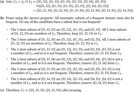
6. The generation of the set of the candidate 3-itemsets, C3, is detailed in Figure 6.3. From the join step, we first get ![]() {{I1, I2, I3}, {I1, I2, I5}, {I1, I3, I5}, {I2, I3, I4}, {I2, I3, I5}, {I2, I4, I5}}. Based on the Apriori property that all subsets of a frequent itemset must also be frequent, we can determine that the four latter candidates cannot possibly be frequent. We therefore remove them from C3, thereby saving the effort of unnecessarily obtaining their counts during the subsequent scan of D to determine L3. Note that when given a candidate k-itemset, we only need to check if its (k − 1)-subsets are frequent since the Apriori algorithm uses a level-wise search strategy. The resulting pruned version of C3 is shown in the first table of the bottom row of Figure 6.2.
{{I1, I2, I3}, {I1, I2, I5}, {I1, I3, I5}, {I2, I3, I4}, {I2, I3, I5}, {I2, I4, I5}}. Based on the Apriori property that all subsets of a frequent itemset must also be frequent, we can determine that the four latter candidates cannot possibly be frequent. We therefore remove them from C3, thereby saving the effort of unnecessarily obtaining their counts during the subsequent scan of D to determine L3. Note that when given a candidate k-itemset, we only need to check if its (k − 1)-subsets are frequent since the Apriori algorithm uses a level-wise search strategy. The resulting pruned version of C3 is shown in the first table of the bottom row of Figure 6.2.
7. The transactions in D are scanned to determine L3, consisting of those candidate 3-itemsets in C3 having minimum support (Figure 6.2).
8. The algorithm uses ![]() to generate a candidate set of 4-itemsets, C4. Although the join results in {{I1, I2, I3, I5}}, itemset {I1, I2, I3, I5} is pruned because its subset {I2, I3, I5} is not frequent. Thus,
to generate a candidate set of 4-itemsets, C4. Although the join results in {{I1, I2, I3, I5}}, itemset {I1, I2, I3, I5} is pruned because its subset {I2, I3, I5} is not frequent. Thus, ![]() , and the algorithm terminates, having found all of the frequent itemsets.
, and the algorithm terminates, having found all of the frequent itemsets.
7![]() is equivalent to
is equivalent to ![]() , since the definition of
, since the definition of ![]() requires the two joining itemsets to share k − 1 = 0 items.
requires the two joining itemsets to share k − 1 = 0 items.
Figure 6.4 shows pseudocode for the Apriori algorithm and its related procedures. Step 1 of Apriori finds the frequent 1-itemsets, L1. In steps 2 through 10, Lk − 1 is used to generate candidates Ck to find Lk for ![]() . The apriori_gen procedure generates the candidates and then uses the Apriori property to eliminate those having a subset that is not frequent (step 3). This procedure is described later. Once all of the candidates have been generated, the database is scanned (step 4). For each transaction, a subset function is used to find all subsets of the transaction that are candidates (step 5), and the count for each of these candidates is accumulated (steps 6 and 7). Finally, all the candidates satisfying the minimum support (step 9) form the set of frequent itemsets, L (step 11). A procedure can then be called to generate association rules from the frequent itemsets. Such a procedure is described in Section 6.2.2.
. The apriori_gen procedure generates the candidates and then uses the Apriori property to eliminate those having a subset that is not frequent (step 3). This procedure is described later. Once all of the candidates have been generated, the database is scanned (step 4). For each transaction, a subset function is used to find all subsets of the transaction that are candidates (step 5), and the count for each of these candidates is accumulated (steps 6 and 7). Finally, all the candidates satisfying the minimum support (step 9) form the set of frequent itemsets, L (step 11). A procedure can then be called to generate association rules from the frequent itemsets. Such a procedure is described in Section 6.2.2.
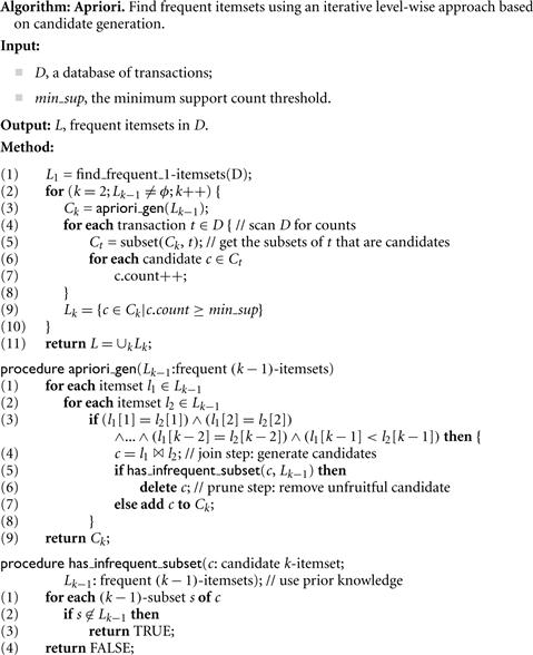
Figure 6.4 Apriori algorithm for discovering frequent itemsets for mining Boolean association rules.
The apriori_gen procedure performs two kinds of actions, namely, join and prune, as described before. In the join component, Lk − 1 is joined with Lk − 1 to generate potential candidates (steps 1–4). The prune component (steps 5–7) employs the Apriori property to remove candidates that have a subset that is not frequent. The test for infrequent subsets is shown in procedure has_infrequent_subset.
6.2.2 Generating Association Rules from Frequent Itemsets
Once the frequent itemsets from transactions in a database D have been found, it is straightforward to generate strong association rules from them (where strong association rules satisfy both minimum support and minimum confidence). This can be done using Eq. (6.4) for confidence, which we show again here for completeness:
![]()
The conditional probability is expressed in terms of itemset support count, where ![]() is the number of transactions containing the itemsets
is the number of transactions containing the itemsets ![]() , and
, and ![]() is the number of transactions containing the itemset A. Based on this equation, association rules can be generated as follows:
is the number of transactions containing the itemset A. Based on this equation, association rules can be generated as follows:
■ For each frequent itemset l, generate all nonempty subsets of l.
■ For every nonempty subset s of l, output the rule “![]() ” if
” if ![]() min_conf, where min_conf is the minimum confidence threshold.
min_conf, where min_conf is the minimum confidence threshold.
Because the rules are generated from frequent itemsets, each one automatically satisfies the minimum support. Frequent itemsets can be stored ahead of time in hash tables along with their counts so that they can be accessed quickly.
Example 6.4
Generating association rules
Let’s try an example based on the transactional data for AllElectronics shown before in Table 6.1. The data contain frequent itemset ![]() {I1, I2, I5}. What are the association rules that can be generated from X? The nonempty subsets of X are {I1, I2}, {I1, I5}, {I2, I5}, {I1}, {I2}, and {I5}. The resulting association rules are as shown below, each listed with its confidence:
{I1, I2, I5}. What are the association rules that can be generated from X? The nonempty subsets of X are {I1, I2}, {I1, I5}, {I2, I5}, {I1}, {I2}, and {I5}. The resulting association rules are as shown below, each listed with its confidence:
{I1, I2}⇒I5, confidence = 2/4 = 50%
{I1, I5}⇒I2, confidence = 2/2 = 100%
{I2, I5}⇒I1, confidence = 2/2 = 100%
I1⇒{I2, I5}, confidence = 2/6 = 33%
If the minimum confidence threshold is, say, 70%, then only the second, third, and last rules are output, because these are the only ones generated that are strong. Note that, unlike conventional classification rules, association rules can contain more than one conjunct in the right side of the rule.
6.2.3 Improving the Efficiency of Apriori
“How can we further improve the efficiency of Apriori-based mining?” Many variations of the Apriori algorithm have been proposed that focus on improving the efficiency of the original algorithm. Several of these variations are summarized as follows:
Hash-based technique (hashing itemsets into corresponding buckets): A hash-based technique can be used to reduce the size of the candidate k-itemsets, Ck, for ![]() . For example, when scanning each transaction in the database to generate the frequent 1-itemsets, L1, we can generate all the 2-itemsets for each transaction, hash (i.e., map) them into the different buckets of a hash table structure, and increase the corresponding bucket counts (Figure 6.5). A 2-itemset with a corresponding bucket count in the hash table that is below the support threshold cannot be frequent and thus should be removed from the candidate set. Such a hash-based technique may substantially reduce the number of candidate k-itemsets examined (especially when
. For example, when scanning each transaction in the database to generate the frequent 1-itemsets, L1, we can generate all the 2-itemsets for each transaction, hash (i.e., map) them into the different buckets of a hash table structure, and increase the corresponding bucket counts (Figure 6.5). A 2-itemset with a corresponding bucket count in the hash table that is below the support threshold cannot be frequent and thus should be removed from the candidate set. Such a hash-based technique may substantially reduce the number of candidate k-itemsets examined (especially when ![]() ).
).
Transaction reduction (reducing the number of transactions scanned in future iterations): A transaction that does not contain any frequent k-itemsets cannot contain any frequent (![]() )-itemsets. Therefore, such a transaction can be marked or removed from further consideration because subsequent database scans for j-itemsets, where
)-itemsets. Therefore, such a transaction can be marked or removed from further consideration because subsequent database scans for j-itemsets, where ![]() , will not need to consider such a transaction.
, will not need to consider such a transaction.
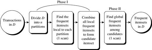
Partitioning (partitioning the data to find candidate itemsets): A partitioning technique can be used that requires just two database scans to mine the frequent itemsets (Figure 6.6). It consists of two phases. In phase I, the algorithm divides the transactions of D into n nonoverlapping partitions. If the minimum relative support threshold for transactions in D is ![]() , then the minimum support count for a partition is
, then the minimum support count for a partition is ![]() × the number of transactions in that partition. For each partition, all the local frequent itemsets (i.e., the itemsets frequent within the partition) are found.
× the number of transactions in that partition. For each partition, all the local frequent itemsets (i.e., the itemsets frequent within the partition) are found.
A local frequent itemset may or may not be frequent with respect to the entire database, D. However, any itemset that is potentially frequent with respect to D must occur as a frequent itemset in at least one of the partitions.8 Therefore, all local frequent itemsets are candidate itemsets with respect to D. The collection of frequent itemsets from all partitions forms the global candidate itemsets with respect to D. In phase II, a second scan of D is conducted in which the actual support of each candidate is assessed to determine the global frequent itemsets. Partition size and the number of partitions are set so that each partition can fit into main memory and therefore be read only once in each phase.
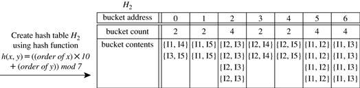
Figure 6.5 Hash table, H2, for candidate 2-itemsets. This hash table was generated by scanning Table 6.1’s transactions while determining L1. If the minimum support count is, say, 3, then the itemsets in buckets 0, 1, 3, and 4 cannot be frequent and so they should not be included in C2.
Sampling (mining on a subset of the given data): The basic idea of the sampling approach is to pick a random sample S of the given data D, and then search for frequent itemsets in S instead of D. In this way, we trade off some degree of accuracy against efficiency. The S sample size is such that the search for frequent itemsets in S can be done in main memory, and so only one scan of the transactions in S is required overall. Because we are searching for frequent itemsets in S rather than in D, it is possible that we will miss some of the global frequent itemsets.
To reduce this possibility, we use a lower support threshold than minimum support to find the frequent itemsets local to S (denoted Ls). The rest of the database is then used to compute the actual frequencies of each itemset in Ls. A mechanism is used to determine whether all the global frequent itemsets are included in Ls. If Ls actually contains all the frequent itemsets in D, then only one scan of D is required. Otherwise, a second pass can be done to find the frequent itemsets that were missed in the first pass. The sampling approach is especially beneficial when efficiency is of utmost importance such as in computationally intensive applications that must be run frequently.
Dynamic itemset counting (adding candidate itemsets at different points during a scan): A dynamic itemset counting technique was proposed in which the database is partitioned into blocks marked by start points. In this variation, new candidate itemsets can be added at any start point, unlike in Apriori, which determines new candidate itemsets only immediately before each complete database scan. The technique uses the count-so-far as the lower bound of the actual count. If the count-so-far passes the minimum support, the itemset is added into the frequent itemset collection and can be used to generate longer candidates. This leads to fewer database scans than with Apriori for finding all the frequent itemsets.
Other variations are discussed in the next chapter.
6.2.4 A Pattern-Growth Approach for Mining Frequent Itemsets
As we have seen, in many cases the Apriori candidate generate-and-test method significantly reduces the size of candidate sets, leading to good performance gain. However, it can suffer from two nontrivial costs:
■ It may still need to generate a huge number of candidate sets. For example, if there are 104 frequent 1-itemsets, the Apriori algorithm will need to generate more than 107 candidate 2-itemsets.
■ It may need to repeatedly scan the whole database and check a large set of candidates by pattern matching. It is costly to go over each transaction in the database to determine the support of the candidate itemsets.
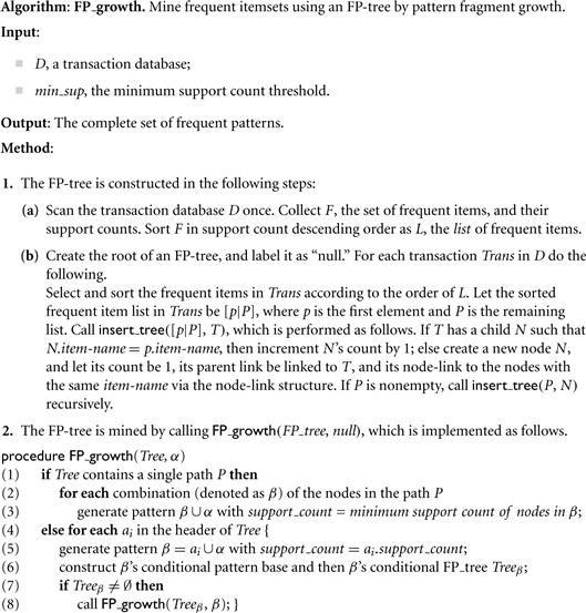
“Can we design a method that mines the complete set of frequent itemsets without such a costly candidate generation process?” An interesting method in this attempt is called frequent pattern growth, or simply FP-growth, which adopts a divide-and-conquer strategy as follows. First, it compresses the database representing frequent items into a frequent pattern tree, or FP-tree, which retains the itemset association information. It then divides the compressed database into a set of conditional databases (a special kind of projected database), each associated with one frequent item or “pattern fragment,” and mines each database separately. For each “pattern fragment,” only its associated data sets need to be examined. Therefore, this approach may substantially reduce the size of the data sets to be searched, along with the “growth” of patterns being examined. You will see how it works in Example 6.5.
Example 6.5
FP-growth (finding frequent itemsets without candidate generation)
We reexamine the mining of transaction database, D, of Table 6.1 in Example 6.3 using the frequent pattern growth approach.
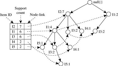
The first scan of the database is the same as Apriori, which derives the set of frequent items (1-itemsets) and their support counts (frequencies). Let the minimum support count be 2. The set of frequent items is sorted in the order of descending support count. This resulting set or list is denoted by L. Thus, we have L = {{I2: 7}, {I1: 6}, {I3: 6}, {I4: 2}, {I5: 2}}.
An FP-tree is then constructed as follows. First, create the root of the tree, labeled with “null.” Scan database D a second time. The items in each transaction are processed in L order (i.e., sorted according to descending support count), and a branch is created for each transaction. For example, the scan of the first transaction, “T100: I1, I2, I5,” which contains three items (I2, I1, I5 in L order), leads to the construction of the first branch of the tree with three nodes, ![]() I2: 1
I2: 1![]() ,
, ![]() I1: 1
I1: 1![]() , and
, and ![]() I5: 1
I5: 1![]() , where I2 is linked as a child to the root, I1 is linked to I2, and I5 is linked to I1. The second transaction, T200, contains the items I2 and I4 in L order, which would result in a branch where I2 is linked to the root and I4 is linked to I2. However, this branch would share a common prefix, I2, with the existing path for T100. Therefore, we instead increment the count of the I2 node by 1, and create a new node,
, where I2 is linked as a child to the root, I1 is linked to I2, and I5 is linked to I1. The second transaction, T200, contains the items I2 and I4 in L order, which would result in a branch where I2 is linked to the root and I4 is linked to I2. However, this branch would share a common prefix, I2, with the existing path for T100. Therefore, we instead increment the count of the I2 node by 1, and create a new node, ![]() I4: 1
I4: 1![]() , which is linked as a child to
, which is linked as a child to ![]() I2: 2
I2: 2![]() . In general, when considering the branch to be added for a transaction, the count of each node along a common prefix is incremented by 1, and nodes for the items following the prefix are created and linked accordingly.
. In general, when considering the branch to be added for a transaction, the count of each node along a common prefix is incremented by 1, and nodes for the items following the prefix are created and linked accordingly.
To facilitate tree traversal, an item header table is built so that each item points to its occurrences in the tree via a chain of node-links. The tree obtained after scanning all the transactions is shown in Figure 6.7 with the associated node-links. In this way, the problem of mining frequent patterns in databases is transformed into that of mining the FP-tree.
The FP-tree is mined as follows. Start from each frequent length-1 pattern (as an initial suffix pattern), construct its conditional pattern base (a “sub-database,” which consists of the set of prefix paths in the FP-tree co-occurring with the suffix pattern), then construct its (conditional) FP-tree, and perform mining recursively on the tree. The pattern growth is achieved by the concatenation of the suffix pattern with the frequent patterns generated from a conditional FP-tree.
Mining of the FP-tree is summarized in Table 6.2 and detailed as follows. We first consider I5, which is the last item in L, rather than the first. The reason for starting at the end of the list will become apparent as we explain the FP-tree mining process. I5 occurs in two FP-tree branches of Figure 6.7. (The occurrences of I5 can easily be found by following its chain of node-links.) The paths formed by these branches are ![]() I2, I1, I5: 1
I2, I1, I5: 1![]() and
and ![]() I2, I1, I3, I5: 1
I2, I1, I3, I5: 1![]() . Therefore, considering I5 as a suffix, its corresponding two prefix paths are
. Therefore, considering I5 as a suffix, its corresponding two prefix paths are ![]() I2, I1: 1
I2, I1: 1![]() and
and ![]() I2, I1, I3: 1
I2, I1, I3: 1![]() , which form its conditional pattern base. Using this conditional pattern base as a transaction database, we build an I5-conditional FP-tree, which contains only a single path,
, which form its conditional pattern base. Using this conditional pattern base as a transaction database, we build an I5-conditional FP-tree, which contains only a single path, ![]() I2: 2, I1: 2
I2: 2, I1: 2![]() ; I3 is not included because its support count of 1 is less than the minimum support count. The single path generates all the combinations of frequent patterns: {I2, I5: 2}, {I1, I5: 2}, {I2, I1, I5: 2}.
; I3 is not included because its support count of 1 is less than the minimum support count. The single path generates all the combinations of frequent patterns: {I2, I5: 2}, {I1, I5: 2}, {I2, I1, I5: 2}.
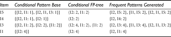
For I4, its two prefix paths form the conditional pattern base, {{I2 I1: 1}, {I2: 1}}, which generates a single-node conditional FP-tree, ![]() I2: 2
I2: 2![]() , and derives one frequent pattern, {I2, I4: 2}.
, and derives one frequent pattern, {I2, I4: 2}.
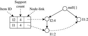
Similar to the preceding analysis, I3’s conditional pattern base is {{I2, I1: 2}, {I2: 2}, {I1: 2}}. Its conditional FP-tree has two branches, ![]() I2: 4, I1: 2
I2: 4, I1: 2![]() and
and ![]() I1: 2
I1: 2![]() , as shown in Figure 6.8, which generates the set of patterns {{I2, I3: 4}, {I1, I3: 4}, {I2, I1, I3: 2}}. Finally, I1’s conditional pattern base is {{I2: 4}}, with an FP-tree that contains only one node,
, as shown in Figure 6.8, which generates the set of patterns {{I2, I3: 4}, {I1, I3: 4}, {I2, I1, I3: 2}}. Finally, I1’s conditional pattern base is {{I2: 4}}, with an FP-tree that contains only one node, ![]() I2: 4
I2: 4![]() , which generates one frequent pattern, {I2, I1: 4}. This mining process is summarized in Figure 6.9.
, which generates one frequent pattern, {I2, I1: 4}. This mining process is summarized in Figure 6.9.
The FP-growth method transforms the problem of finding long frequent patterns into searching for shorter ones in much smaller conditional databases recursively and then concatenating the suffix. It uses the least frequent items as a suffix, offering good selectivity. The method substantially reduces the search costs.
When the database is large, it is sometimes unrealistic to construct a main memory-based FP-tree. An interesting alternative is to first partition the database into a set of projected databases, and then construct an FP-tree and mine it in each projected database. This process can be recursively applied to any projected database if its FP-tree still cannot fit in main memory.
A study of the FP-growth method performance shows that it is efficient and scalable for mining both long and short frequent patterns, and is about an order of magnitude faster than the Apriori algorithm.
6.2.5 Mining Frequent Itemsets Using the Vertical Data Format
Both the Apriori and FP-growth methods mine frequent patterns from a set of transactions in TID-itemset format (i.e., ![]() ), where TID is a transaction ID and itemset is the set of items bought in transaction TID. This is known as the horizontal data format. Alternatively, data can be presented in item-TID_set format (i.e.,
), where TID is a transaction ID and itemset is the set of items bought in transaction TID. This is known as the horizontal data format. Alternatively, data can be presented in item-TID_set format (i.e., ![]() , where item is an item name, and TID_set is the set of transaction identifiers containing the item. This is known as the vertical data format.
, where item is an item name, and TID_set is the set of transaction identifiers containing the item. This is known as the vertical data format.
In this subsection, we look at how frequent itemsets can also be mined efficiently using vertical data format, which is the essence of the Eclat (Equivalence Class Transformation) algorithm.
Example 6.6 illustrates the process of mining frequent itemsets by exploring the vertical data format. First, we transform the horizontally formatted data into the vertical format by scanning the data set once. The support count of an itemset is simply the length of the TID_set of the itemset. Starting with ![]() , the frequent k-itemsets can be used to construct the candidate (k + 1)-itemsets based on the Apriori property. The computation is done by intersection of the TID_sets of the frequent k-itemsets to compute the TID_sets of the corresponding (k + 1)-itemsets. This process repeats, with k incremented by 1 each time, until no frequent itemsets or candidate itemsets can be found.
, the frequent k-itemsets can be used to construct the candidate (k + 1)-itemsets based on the Apriori property. The computation is done by intersection of the TID_sets of the frequent k-itemsets to compute the TID_sets of the corresponding (k + 1)-itemsets. This process repeats, with k incremented by 1 each time, until no frequent itemsets or candidate itemsets can be found.
Besides taking advantage of the Apriori property in the generation of candidate (k + 1)-itemset from frequent k-itemsets, another merit of this method is that there is no need to scan the database to find the support of (k + 1)-itemsets (for ![]() ). This is because the TID_set of each k-itemset carries the complete information required for counting such support. However, the TID_sets can be quite long, taking substantial memory space as well as computation time for intersecting the long sets.
). This is because the TID_set of each k-itemset carries the complete information required for counting such support. However, the TID_sets can be quite long, taking substantial memory space as well as computation time for intersecting the long sets.
To further reduce the cost of registering long TID_sets, as well as the subsequent costs of intersections, we can use a technique called diffset, which keeps track of only the differences of the TID_sets of a (k + 1)-itemset and a corresponding k-itemset. For instance, in Example 6.6 we have {I1} = {T100, T400, T500, T700, T800, T900} and {I1, I2} = {T100, T400, T800, T900}. The diffset between the two is diffset ({I1, I2}, {I1}) = {T500, T700}. Thus, rather than recording the four TIDs that make up the intersection of {I1} and {I2}, we can instead use diffset to record just two TIDs, indicating the difference between {I1} and {I1, I2}. Experiments show that in certain situations, such as when the data set contains many dense and long patterns, this technique can substantially reduce the total cost of vertical format mining of frequent itemsets.
6.2.6 Mining Closed and Max Patterns
In Section 6.1.2 we saw how frequent itemset mining may generate a huge number of frequent itemsets, especially when the min_sup threshold is set low or when there exist long patterns in the data set. Example 6.2 showed that closed frequent itemsets9 can substantially reduce the number of patterns generated in frequent itemset mining while preserving the complete information regarding the set of frequent itemsets. That is, from the set of closed frequent itemsets, we can easily derive the set of frequent itemsets and their support. Thus, in practice, it is more desirable to mine the set of closed frequent itemsets rather than the set of all frequent itemsets in most cases.
“How can we mine closed frequent itemsets?” A na ve approach would be to first mine the complete set of frequent itemsets and then remove every frequent itemset that is a proper subset of, and carries the same support as, an existing frequent itemset. However, this is quite costly. As shown in Example 6.2, this method would have to first derive ![]() frequent itemsets to obtain a length-100 frequent itemset, all before it could begin to eliminate redundant itemsets. This is prohibitively expensive. In fact, there exist only a very small number of closed frequent itemsets in Example 6.2’s data set.
frequent itemsets to obtain a length-100 frequent itemset, all before it could begin to eliminate redundant itemsets. This is prohibitively expensive. In fact, there exist only a very small number of closed frequent itemsets in Example 6.2’s data set.
A recommended methodology is to search for closed frequent itemsets directly during the mining process. This requires us to prune the search space as soon as we can identify the case of closed itemsets during mining. Pruning strategies include the following:
Item merging: If every transaction containing a frequent itemset X also contains an itemset Y but not any proper superset of Y, then ![]() forms a frequent closed itemset and there is no need to search for any itemset containing X but no Y.
forms a frequent closed itemset and there is no need to search for any itemset containing X but no Y.
For example, in Table 6.2 of Example 6.5, the projected conditional database for prefix itemset {I5:2} is {{I2, I1}, {I2, I1, I3}}, from which we can see that each of its transactions contains itemset {I2, I1} but no proper superset of {I2, I1}. Itemset {I2, I1} can be merged with {I5} to form the closed itemset, {I5, I2, I1: 2}, and we do not need to mine for closed itemsets that contain I5 but not {I2, I1}.
Sub-itemset pruning: If a frequent itemset X is a proper subset of an already found frequent closed itemset Y and support_count(X) = support_count(Y), then X and all of X’s descendants in the set enumeration tree cannot be frequent closed itemsets and thus can be pruned.
Similar to Example 6.2, suppose a transaction database has only two transactions: {![]() ,
, ![]() }, and the minimum support count is min_sup = 2. The projection on the first item,
}, and the minimum support count is min_sup = 2. The projection on the first item, ![]() , derives the frequent itemset, {
, derives the frequent itemset, {![]()
![]() }, based on the itemset merging optimization. Because support ({
}, based on the itemset merging optimization. Because support ({![]() }) = support ({
}) = support ({![]() }) = 2, and {
}) = 2, and {![]() } is a proper subset of {
} is a proper subset of {![]() }, there is no need to examine
}, there is no need to examine ![]() and its projected database. Similar pruning can be done for
and its projected database. Similar pruning can be done for ![]() as well. Thus, the mining of closed frequent itemsets in this data set terminates after mining
as well. Thus, the mining of closed frequent itemsets in this data set terminates after mining ![]() ’s projected database.
’s projected database.
Item skipping: In the depth-first mining of closed itemsets, at each level, there will be a prefix itemset X associated with a header table and a projected database. If a local frequent item p has the same support in several header tables at different levels, we can safely prune p from the header tables at higher levels.
Consider, for example, the previous transaction database having only two transactions: {![]() ,
, ![]() }, where
}, where ![]() . Because
. Because ![]() in
in ![]() ’s projected database has the same support as
’s projected database has the same support as ![]() in the global header table,
in the global header table, ![]() can be pruned from the global header table. Similar pruning can be done for
can be pruned from the global header table. Similar pruning can be done for ![]() . There is no need to mine anything more after mining
. There is no need to mine anything more after mining ![]() ’s projected database.
’s projected database.
Besides pruning the search space in the closed itemset mining process, another important optimization is to perform efficient checking of each newly derived frequent itemset to see whether it is closed. This is because the mining process cannot ensure that every generated frequent itemset is closed.
When a new frequent itemset is derived, it is necessary to perform two kinds of closure checking: (1) superset checking, which checks if this new frequent itemset is a superset of some already found closed itemsets with the same support, and (2) subset checking, which checks whether the newly found itemset is a subset of an already found closed itemset with the same support.
If we adopt the item merging pruning method under a divide-and-conquer framework, then the superset checking is actually built-in and there is no need to explicitly perform superset checking. This is because if a frequent itemset ![]() is found later than itemset X, and carries the same support as X, it must be in X’s projected database and must have been generated during itemset merging.
is found later than itemset X, and carries the same support as X, it must be in X’s projected database and must have been generated during itemset merging.
To assist in subset checking, a compressed pattern-tree can be constructed to maintain the set of closed itemsets mined so far. The pattern-tree is similar in structure to the FP-tree except that all the closed itemsets found are stored explicitly in the corresponding tree branches. For efficient subset checking, we can use the following property: If the current itemset ![]() can be subsumed by another already found closed itemset
can be subsumed by another already found closed itemset ![]() , then (1)
, then (1) ![]() and
and ![]() have the same support, (2) the length of
have the same support, (2) the length of ![]() is smaller than that of
is smaller than that of ![]() , and (3) all of the items in
, and (3) all of the items in ![]() are contained in
are contained in ![]() .
.
Based on this property, a two-level hash index structure can be built for fast accessing of the pattern-tree: The first level uses the identifier of the last item in ![]() as a hash key (since this identifier must be within the branch of
as a hash key (since this identifier must be within the branch of ![]() ), and the second level uses the support of
), and the second level uses the support of ![]() as a hash key (since
as a hash key (since ![]() and
and ![]() have the same support). This will substantially speed up the subset checking process.
have the same support). This will substantially speed up the subset checking process.
This discussion illustrates methods for efficient mining of closed frequent itemsets. “Can we extend these methods for efficient mining of maximal frequent itemsets?” Because maximal frequent itemsets share many similarities with closed frequent itemsets, many of the optimization techniques developed here can be extended to mining maximal frequent itemsets. However, we leave this method as an exercise for interested readers.