
6.3 Which Patterns Are Interesting?—Pattern Evaluation Methods
Most association rule mining algorithms employ a support–confidence framework. Although minimum support and confidence thresholds help weed out or exclude the exploration of a good number of uninteresting rules, many of the rules generated are still not interesting to the users. Unfortunately, this is especially true when mining at low support thresholds or mining for long patterns. This has been a major bottleneck for successful application of association rule mining.
In this section, we first look at how even strong association rules can be uninteresting and misleading (Section 6.3.1). We then discuss how the support–confidence framework can be supplemented with additional interestingness measures based on correlation analysis (Section 6.3.2). Section 6.3.3 presents additional pattern evaluation measures. It then provides an overall comparison of all the measures discussed here. By the end, you will learn which pattern evaluation measures are most effective for the discovery of only interesting rules.
6.3.1 Strong Rules Are Not Necessarily Interesting
Whether or not a rule is interesting can be assessed either subjectively or objectively. Ultimately, only the user can judge if a given rule is interesting, and this judgment, being subjective, may differ from one user to another. However, objective interestingness measures, based on the statistics “behind” the data, can be used as one step toward the goal of weeding out uninteresting rules that would otherwise be presented to the user.
“How can we tell which strong association rules are really interesting?” Let’s examine the following example.
Example 6.7
A misleading “strong” association rule
Suppose we are interested in analyzing transactions at AllElectronics with respect to the purchase of computer games and videos. Let game refer to the transactions containing computer games, and video refer to those containing videos. Of the 10,000 transactions analyzed, the data show that 6000 of the customer transactions included computer games, while 7500 included videos, and 4000 included both computer games and videos. Suppose that a data mining program for discovering association rules is run on the data, using a minimum support of, say, 30% and a minimum confidence of 60%. The following association rule is discovered:
![]() (6.6)
(6.6)
Rule (6.6) is a strong association rule and would therefore be reported, since its support value of ![]() and confidence value of
and confidence value of ![]() satisfy the minimum support and minimum confidence thresholds, respectively. However, Rule (6.6) is misleading because the probability of purchasing videos is 75%, which is even larger than 66%. In fact, computer games and videos are negatively associated because the purchase of one of these items actually decreases the likelihood of purchasing the other. Without fully understanding this phenomenon, we could easily make unwise business decisions based on Rule (6.6).
satisfy the minimum support and minimum confidence thresholds, respectively. However, Rule (6.6) is misleading because the probability of purchasing videos is 75%, which is even larger than 66%. In fact, computer games and videos are negatively associated because the purchase of one of these items actually decreases the likelihood of purchasing the other. Without fully understanding this phenomenon, we could easily make unwise business decisions based on Rule (6.6).
Example 6.7 also illustrates that the confidence of a rule ![]() can be deceiving. It does not measure the real strength (or lack of strength) of the correlation and implication between A and B. Hence, alternatives to the support–confidence framework can be useful in mining interesting data relationships.
can be deceiving. It does not measure the real strength (or lack of strength) of the correlation and implication between A and B. Hence, alternatives to the support–confidence framework can be useful in mining interesting data relationships.
6.3.2 From Association Analysis to Correlation Analysis
As we have seen so far, the support and confidence measures are insufficient at filtering out uninteresting association rules. To tackle this weakness, a correlation measure can be used to augment the support–confidence framework for association rules. This leads to correlation rules of the form
![]() (6.7)
(6.7)
That is, a correlation rule is measured not only by its support and confidence but also by the correlation between itemsets A and B. There are many different correlation measures from which to choose. In this subsection, we study several correlation measures to determine which would be good for mining large data sets.
Lift is a simple correlation measure that is given as follows. The occurrence of itemset A is independent of the occurrence of itemset B if ![]() ; otherwise, itemsets A and B are dependent and correlated as events. This definition can easily be extended to more than two itemsets. The lift between the occurrence of A and B can be measured by computing
; otherwise, itemsets A and B are dependent and correlated as events. This definition can easily be extended to more than two itemsets. The lift between the occurrence of A and B can be measured by computing
![]() (6.8)
(6.8)
If the resulting value of Eq. (6.8) is less than 1, then the occurrence of A is negatively correlated with the occurrence of B, meaning that the occurrence of one likely leads to the absence of the other one. If the resulting value is greater than 1, then A and B are positively correlated, meaning that the occurrence of one implies the occurrence of the other. If the resulting value is equal to 1, then A and B are independent and there is no correlation between them.
Equation (6.8) is equivalent to ![]() , or
, or ![]() , which is also referred to as the lift of the association (or correlation) rule
, which is also referred to as the lift of the association (or correlation) rule ![]() . In other words, it assesses the degree to which the occurrence of one “lifts” the occurrence of the other. For example, if A corresponds to the sale of computer games and B corresponds to the sale of videos, then given the current market conditions, the sale of games is said to increase or “lift” the likelihood of the sale of videos by a factor of the value returned by Eq. (6.8).
. In other words, it assesses the degree to which the occurrence of one “lifts” the occurrence of the other. For example, if A corresponds to the sale of computer games and B corresponds to the sale of videos, then given the current market conditions, the sale of games is said to increase or “lift” the likelihood of the sale of videos by a factor of the value returned by Eq. (6.8).
Let’s go back to the computer game and video data of Example 6.7.
Example 6.8
Correlation analysis using lift
To help filter out misleading “strong” associations of the form ![]() from the data of Example 6.7, we need to study how the two itemsets, A and B, are correlated. Let
from the data of Example 6.7, we need to study how the two itemsets, A and B, are correlated. Let ![]() refer to the transactions of Example 6.7 that do not contain computer games, and
refer to the transactions of Example 6.7 that do not contain computer games, and ![]() refer to those that do not contain videos. The transactions can be summarized in a contingency table, as shown in Table 6.6.
refer to those that do not contain videos. The transactions can be summarized in a contingency table, as shown in Table 6.6.
Table 6.6
2 × 2 Contingency Table Summarizing the Transactions with Respect to Game and Video Purchases
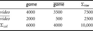
From the table, we can see that the probability of purchasing a computer game is ![]() , the probability of purchasing a video is
, the probability of purchasing a video is ![]() , and the probability of purchasing both is
, and the probability of purchasing both is ![]() . By Eq. (6.8), the lift of Rule (6.6) is
. By Eq. (6.8), the lift of Rule (6.6) is ![]() . Because this value is less than 1, there is a negative correlation between the occurrence of {game} and {video}. The numerator is the likelihood of a customer purchasing both, while the denominator is what the likelihood would have been if the two purchases were completely independent. Such a negative correlation cannot be identified by a support–confidence framework.
. Because this value is less than 1, there is a negative correlation between the occurrence of {game} and {video}. The numerator is the likelihood of a customer purchasing both, while the denominator is what the likelihood would have been if the two purchases were completely independent. Such a negative correlation cannot be identified by a support–confidence framework.
The second correlation measure that we study is the ![]() measure, which was introduced in Chapter 3 (Eq. 3.1). To compute the
measure, which was introduced in Chapter 3 (Eq. 3.1). To compute the ![]() value, we take the squared difference between the observed and expected value for a slot (A and B pair) in the contingency table, divided by the expected value. This amount is summed for all slots of the contingency table. Let’s perform a
value, we take the squared difference between the observed and expected value for a slot (A and B pair) in the contingency table, divided by the expected value. This amount is summed for all slots of the contingency table. Let’s perform a ![]() analysis of Example 6.8.
analysis of Example 6.8.
Example 6.9
Correlation analysis using χ2
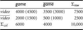
To compute the correlation using ![]() analysis for nominal data, we need the observed value and expected value (displayed in parenthesis) for each slot of the contingency table, as shown in Table 6.7. From the table, we can compute the
analysis for nominal data, we need the observed value and expected value (displayed in parenthesis) for each slot of the contingency table, as shown in Table 6.7. From the table, we can compute the ![]() value as follows:
value as follows:
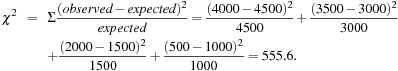
Because the ![]() value is greater than 1, and the observed value of the slot (game, video) = 4000, which is less than the expected value of 4500, buying game and buying video are negatively correlated. This is consistent with the conclusion derived from the analysis of the lift measure in Example 6.8.
value is greater than 1, and the observed value of the slot (game, video) = 4000, which is less than the expected value of 4500, buying game and buying video are negatively correlated. This is consistent with the conclusion derived from the analysis of the lift measure in Example 6.8.
6.3.3 A Comparison of Pattern Evaluation Measures
The above discussion shows that instead of using the simple support–confidence framework to evaluate frequent patterns, other measures, such as lift and ![]() , often disclose more intrinsic pattern relationships. How effective are these measures? Should we also consider other alternatives?
, often disclose more intrinsic pattern relationships. How effective are these measures? Should we also consider other alternatives?
Researchers have studied many pattern evaluation measures even before the start of in-depth research on scalable methods for mining frequent patterns. Recently, several other pattern evaluation measures have attracted interest. In this subsection, we present four such measures: all_confidence, max_confidence, Kulczynski, and cosine. We’ll then compare their effectiveness with respect to one another and with respect to the lift and ![]() measures.
measures.
Given two itemsets, A and B, the all_confidence measure of A and B is defined as
![]() (6.9)
(6.9)
where max {sup (A), sup (B)} is the maximum support of the itemsets A and B. Thus, ![]() is also the minimum confidence of the two association rules related to A and B, namely, “
is also the minimum confidence of the two association rules related to A and B, namely, “![]() ” and “
” and “![]() .”
.”
Given two itemsets, A and B, the max_confidence measure of A and B is defined as
![]() (6.10)
(6.10)
The max_conf measure is the maximum confidence of the two association rules, “![]() ” and “
” and “![]() .”
.”
Given two itemsets, A and B, the Kulczynski measure of A and B (abbreviated as Kulc) is defined as
![]() (6.11)
(6.11)
It was proposed in 1927 by Polish mathematician S. Kulczynski. It can be viewed as an average of two confidence measures. That is, it is the average of two conditional probabilities: the probability of itemset B given itemset A, and the probability of itemset A given itemset B.
Finally, given two itemsets, A and B, the cosine measure of A and B is defined as
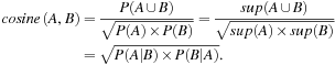 (6.12)
The cosine measure can be viewed as a harmonized lift measure: The two formulae are similar except that for cosine, the square root is taken on the product of the probabilities of A and B. This is an important difference, however, because by taking the square root, the cosine value is only influenced by the supports of A, B, and ![]() , and not by the total number of transactions.
, and not by the total number of transactions.
Each of these four measures defined has the following property: Its value is only influenced by the supports of A, B, and ![]() , or more exactly, by the conditional probabilities of
, or more exactly, by the conditional probabilities of ![]() and
and ![]() , but not by the total number of transactions. Another common property is that each measure ranges from 0 to 1, and the higher the value, the closer the relationship between A and B.
, but not by the total number of transactions. Another common property is that each measure ranges from 0 to 1, and the higher the value, the closer the relationship between A and B.
Now, together with lift and ![]() , we have introduced in total six pattern evaluation measures. You may wonder, “Which is the best in assessing the discovered pattern relationships?” To answer this question, we examine their performance on some typical data sets.
, we have introduced in total six pattern evaluation measures. You may wonder, “Which is the best in assessing the discovered pattern relationships?” To answer this question, we examine their performance on some typical data sets.
Example 6.10
Comparison of six pattern evaluation measures on typical data sets
The relationships between the purchases of two items, milk and coffee, can be examined by summarizing their purchase history in Table 6.8, a 2 × 2 contingency table, where an entry such as mc represents the number of transactions containing both milk and coffee.
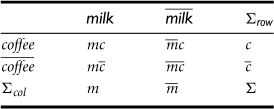
Table 6.9 shows a set of transactional data sets with their corresponding contingency tables and the associated values for each of the six evaluation measures. Let’s first examine the first four data sets, D1 through D4. From the table, we see that m and c are positively associated in D1 and D2, negatively associated in D3, and neutral in D4. For D1 and D2, m and c are positively associated because mc (10,000) is considerably greater than ![]() (1000) and
(1000) and ![]() (1000). Intuitively, for people who bought milk (
(1000). Intuitively, for people who bought milk (![]() ), it is very likely that they also bought coffee (
), it is very likely that they also bought coffee (![]() ), and vice versa.
), and vice versa.
Table 6.9
Comparison of Six Pattern Evaluation Measures Using Contingency Tables for a Variety of Data Sets
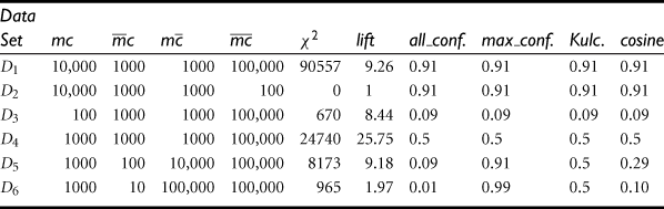
The results of the four newly introduced measures show that m and c are strongly positively associated in both data sets by producing a measure value of 0.91. However, lift and ![]() generate dramatically different measure values for D1 and D2 due to their sensitivity to
generate dramatically different measure values for D1 and D2 due to their sensitivity to ![]() . In fact, in many real-world scenarios,
. In fact, in many real-world scenarios, ![]() is usually huge and unstable. For example, in a market basket database, the total number of transactions could fluctuate on a daily basis and overwhelmingly exceed the number of transactions containing any particular itemset. Therefore, a good interestingness measure should not be affected by transactions that do not contain the itemsets of interest; otherwise, it would generate unstable results, as illustrated in D1 and D2.
is usually huge and unstable. For example, in a market basket database, the total number of transactions could fluctuate on a daily basis and overwhelmingly exceed the number of transactions containing any particular itemset. Therefore, a good interestingness measure should not be affected by transactions that do not contain the itemsets of interest; otherwise, it would generate unstable results, as illustrated in D1 and D2.
Similarly, in D3, the four new measures correctly show that m and c are strongly negatively associated because the m to c ratio equals the mc to m ratio, that is, ![]() . However, lift and
. However, lift and ![]() both contradict this in an incorrect way: Their values for D2 are between those for D1 and D3.
both contradict this in an incorrect way: Their values for D2 are between those for D1 and D3.
For data set D4, both lift and ![]() indicate a highly positive association between m and c, whereas the others indicate a “neutral” association because the ratio of mc to
indicate a highly positive association between m and c, whereas the others indicate a “neutral” association because the ratio of mc to ![]() equals the ratio of mc to
equals the ratio of mc to ![]() , which is 1. This means that if a customer buys coffee (or milk), the probability that he or she will also purchase milk (or coffee) is exactly 50%.
, which is 1. This means that if a customer buys coffee (or milk), the probability that he or she will also purchase milk (or coffee) is exactly 50%.
“Why are lift and ![]() so poor at distinguishing pattern association relationships in the previous transactional data sets?” To answer this, we have to consider the null- transactions. A null-transaction is a transaction that does not contain any of the itemsets being examined. In our example,
so poor at distinguishing pattern association relationships in the previous transactional data sets?” To answer this, we have to consider the null- transactions. A null-transaction is a transaction that does not contain any of the itemsets being examined. In our example, ![]() represents the number of null-transactions. Lift and
represents the number of null-transactions. Lift and ![]() have difficulty distinguishing interesting pattern association relationships because they are both strongly influenced by
have difficulty distinguishing interesting pattern association relationships because they are both strongly influenced by ![]() . Typically, the number of null-transactions can outweigh the number of individual purchases because, for example, many people may buy neither milk nor coffee. On the other hand, the other four measures are good indicators of interesting pattern associations because their definitions remove the influence of
. Typically, the number of null-transactions can outweigh the number of individual purchases because, for example, many people may buy neither milk nor coffee. On the other hand, the other four measures are good indicators of interesting pattern associations because their definitions remove the influence of ![]() (i.e., they are not influenced by the number of null-transactions).
(i.e., they are not influenced by the number of null-transactions).
This discussion shows that it is highly desirable to have a measure that has a value that is independent of the number of null-transactions. A measure is null-invariant if its value is free from the influence of null-transactions. Null-invariance is an important property for measuring association patterns in large transaction databases. Among the six discussed measures in this subsection, only lift and ![]() are not null-invariant measures.
are not null-invariant measures.
“Among the all_confidence, max_confidence, Kulczynski, and cosine measures, which is best at indicating interesting pattern relationships?”
To answer this question, we introduce the imbalance ratio (IR), which assesses the imbalance of two itemsets, A and B, in rule implications. It is defined as
![]() (6.13)
(6.13)
where the numerator is the absolute value of the difference between the support of the itemsets A and B, and the denominator is the number of transactions containing A or B. If the two directional implications between A and B are the same, then ![]() will be zero. Otherwise, the larger the difference between the two, the larger the imbalance ratio. This ratio is independent of the number of null-transactions and independent of the total number of transactions.
will be zero. Otherwise, the larger the difference between the two, the larger the imbalance ratio. This ratio is independent of the number of null-transactions and independent of the total number of transactions.
Let’s continue examining the remaining data sets in Example 6.10.
Example 6.11
Comparing null-invariant measures in pattern evaluation
Although the four measures introduced in this section are null-invariant, they may present dramatically different values on some subtly different data sets. Let’s examine data sets D5 and D6, shown earlier in Table 6.9, where the two events m and c have unbalanced conditional probabilities. That is, the ratio of mc to c is greater than 0.9. This means that knowing that c occurs should strongly suggest that m occurs also. The ratio of mc to m is less than 0.1, indicating that m implies that c is quite unlikely to occur. The all_confidence and cosine measures view both cases as negatively associated and the Kulc measure views both as neutral. The max_confidence measure claims strong positive associations for these cases. The measures give very diverse results!
“Which measure intuitively reflects the true relationship between the purchase of milk and coffee?” Due to the “balanced” skewness of the data, it is difficult to argue whether the two data sets have positive or negative association. From one point of view, only ![]() % of milk-related transactions contain coffee in D5 and this percentage is
% of milk-related transactions contain coffee in D5 and this percentage is ![]() % in D6, both indicating a negative association. On the other hand,
% in D6, both indicating a negative association. On the other hand, ![]() % of transactions in D5 (i.e.,
% of transactions in D5 (i.e., ![]() ) and 9% in D6 (i.e.,
) and 9% in D6 (i.e., ![]() ) containing coffee contain milk as well, which indicates a positive association between milk and coffee. These draw very different conclusions.
) containing coffee contain milk as well, which indicates a positive association between milk and coffee. These draw very different conclusions.
For such “balanced” skewness, it could be fair to treat it as neutral, as Kulc does, and in the meantime indicate its skewness using the imbalance ratio (IR). According to Eq. (6.13), for D4 we have ![]() , a perfectly balanced case; for D5,
, a perfectly balanced case; for D5, ![]() , a rather imbalanced case; whereas for D6,
, a rather imbalanced case; whereas for D6, ![]() , a very skewed case. Therefore, the two measures, Kulc and
, a very skewed case. Therefore, the two measures, Kulc and ![]() , work together, presenting a clear picture for all three data sets, D4 through D6.
, work together, presenting a clear picture for all three data sets, D4 through D6.
In summary, the use of only support and confidence measures to mine associations may generate a large number of rules, many of which can be uninteresting to users. Instead, we can augment the support–confidence framework with a pattern interestingness measure, which helps focus the mining toward rules with strong pattern relationships. The added measure substantially reduces the number of rules generated and leads to the discovery of more meaningful rules. Besides those introduced in this section, many other interestingness measures have been studied in the literature. Unfortunately, most of them do not have the null-invariance property. Because large data sets typically have many null-transactions, it is important to consider the null-invariance property when selecting appropriate interestingness measures for pattern evaluation. Among the four null-invariant measures studied here, namely all_confidence, max_confidence, Kulc, and cosine, we recommend using Kulc in conjunction with the imbalance ratio.