Search in book...
Toggle Font Controls
Create new playlist

Name your new playlist

Playlist description (optional)
Sign In

Email address

Password

Forgot Password?

or

Continue with Facebook

Continue with Google
Sign Up

Full Name

Email address

Confirm Email Address

Password

or

Continue with Facebook

Continue with Google

7.4 A Gallery of Solution Curves of Linear Systems

In the preceding section we saw that the eigenvalues and eigenvectors of the n×n $n \times n$ matrix A are of central importance to the solutions of the homogeneous linear constant-coefficient system

x' = A x .

$x^{′} = A x .$ (1)

Indeed, according to Theorem 1 from Section 7.3, if λ $λ$ is an eigenvalue of A and v is an eigenvector of A associated with λ, $λ,$ then

x (t) = v e λ t

$x (t) = v e^{λ t}$ (2)

is a nontrivial solution of the system (1). Moreover, if A has n linearly independent eigenvectors v1, v2, …, $v_{1}, v_{2}, \dots,$ vn $v_{n}$ associated with its n eigenvalues λ1, λ2, …, $λ_{1}, λ_{2}, \dots,$ λn, $λ_{n},$ then in fact all solutions of the system (1) are given by linear combinations

x (t) = c 1 v 1 e λ 1 t + c 2 v 2 e λ 2 t + \dots + c n v n e λ n t,

$x (t) = c_{1} v_{1} e^{λ_{1} t} + c_{2} v_{2} e^{λ_{2} t} + \dots + c_{n} v_{n} e^{λ_{n} t},$ (3)

where c1,c2,…,cn $c_{1}, c_{2}, \dots, c_{n}$ are arbitrary constants. If the eigenvalues include complex conjugate pairs, then we can obtain a real-valued general solution from Eq. (3) by taking real and imaginary parts of the terms in (3) corresponding to the complex eigenvalues.

Our goal in this section is to gain a geometric understanding of the role that the eigenvalues and eigenvectors of the matrix A play in the solutions of the system (1). We will see, illustrating primarily with the case n=2, $n = 2,$ that particular arrangements of eigenvalues and eigenvectors correspond to identifiable patterns—“fingerprints,” so to speak—in the phase plane portrait of the system (1). Just as in algebra we learn to recognize when an equation in x and y corresponds to a line or parabola, we can predict the general appearance of the solution curves of the system (1) from the eigenvalues and eigenvectors of the matrix A. By considering various cases for these eigenvalues and eigenvectors we will create a “gallery”—Figure 7.4.16 appearing at the end of this section—of typical phase plane portraits that gives, in essence, a complete catalog of the geometric behaviors that the solutions of a 2×2 $2 \times 2$ homogeneous linear constant-coefficient system can exhibit. This will help us analyze not only systems of the form (1), but also more complicated systems that can be approximated by linear systems, a topic we explore in Section 9.2.

Systems of Dimension n=2

Until stated otherwise, we henceforth assume that n=2, $n = 2,$ so that the eigenvalues of the matrix A are λ1 $λ_{1}$ and λ2. $λ_{2} .$ According to Theorem 2 of Section 6.2, if λ1 $λ_{1}$ and λ2 $λ_{2}$ are distinct, then the associated eigenvectors v1 $v_{1}$ and v2 $v_{2}$ of A are linearly independent. In this event, the general solution of the system (1) is given by

x (t) = c 1 v 1 e λ 1 t + c 2 v 2 e λ 2 t

$x (t) = c_{1} v_{1} e^{λ_{1} t} + c_{2} v_{2} e^{λ_{2} t}$ (4)

if λ1 $λ_{1}$ and λ2 $λ_{2}$ are real, and by

x (t) = c 1 e p t (a cos q t - b sin q t) + c 2 e p t (b cos q t + a sin q t)

$x (t) = c_{1} e^{p t} (a \cos q t - b \sin q t) + c_{2} e^{p t} (b \cos q t + a \sin q t)$ (5)

if λ1 $λ_{1}$ and λ2 $λ_{2}$ are the complex conjugate numbers p±iq $p \pm i q$ ; here the vectors a and b are the real and imaginary parts, respectively, of a (complex-valued) eigenvector of A associated with the eigenvalue p±iq. $p \pm i q .$ If instead λ1 $λ_{1}$ and λ2 $λ_{2}$ are equal (to a common value λ, $λ,$ say), then as we will see in Section 7.6, the matrix A may or may not have two linearly independent eigenvectors v1 $v_{1}$ and v2. $v_{2} .$ If it does, then the eigenvalue method of Section 7.3 applies once again, and the general solution of the system (1) is given by the linear combination

x (t) = c 1 v 1 e λ t + c 2 v 2 e λ t

$x (t) = c_{1} v_{1} e^{λ t} + c_{2} v_{2} e^{λ t}$ (6)

as before. If A does not have two linearly independent eigenvectors, then—as we will see—we can find a vector v2 $v_{2}$ such that the general solution of the system (1) is given by

x (t) = c 1 v 1 e λ t + c 2 (v 1 t + v 2) e λ t,

$x (t) = c_{1} v_{1} e^{λ t} + c_{2} (v_{1} t + v_{2}) e^{λ t},$ (7)

where v1 $v_{1}$ is an eigenvector of A associated with the lone eigenvalue λ. $λ .$ The nature of the vector v2 $v_{2}$ and other details of the general solution in (7) will be discussed in Section 7.6, but we include this case here in order to make our gallery complete.

With this algebraic background in place, we begin our analysis of the solution curves of the system (1). First we assume that the eigenvalues λ1 $λ_{1}$ and λ2 $λ_{2}$ of the matrix A are real, and subsequently we take up the case where λ1 $λ_{1}$ and λ2 $λ_{2}$ are complex conjugates.

Real Eigenvalues

We will divide the case where λ1 $λ_{1}$ and λ2 $λ_{2}$ are real into the following possibilities:

Distinct eigenvalues

Nonzero and of opposite sign (λ1<0<λ2 $λ_{1} < 0 < λ_{2}$ )
Both negative (λ1<λ2<0 $λ_{1} < λ_{2} < 0$ )
Both positive (0<λ2<λ1 $0 < λ_{2} < λ_{1}$ )
One zero and one negative (λ1<λ2=0 $λ_{1} < λ_{2} = 0$ )
One zero and one positive (0=λ2<λ1 $0 = λ_{2} < λ_{1}$ )

Repeated eigenvalue

Positive (λ1=λ2>0 $λ_{1} = λ_{2} > 0$ )
Negative (λ1=λ2<0 $λ_{1} = λ_{2} < 0$ )
Zero (λ1=λ2=0 $λ_{1} = λ_{2} = 0$ )

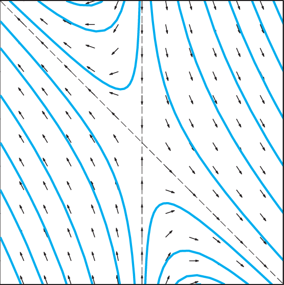
Saddle Points

Nonzero Distinct Eigenvalues of Opposite Sign: The key observation when λ1<0<λ2 $λ_{1} < 0 < λ_{2}$ is that the positive scalar factors eλ1t $e^{λ_{1} t}$ and eλ2t $e^{λ_{2} t}$ in the general solution

x (t) = c 1 v 1 e λ 1 t + c 2 v 2 e λ 2 t

$x (t) = c_{1} v_{1} e^{λ_{1} t} + c_{2} v_{2} e^{λ_{2} t}$ (4)

of the system x'=Ax $x ′ = A x$ move in opposite directions (on the real line) as t varies. For example, as t grows large and positive, eλ2t $e^{λ_{2} t}$ grows large, because λ2>0, $λ_{2} > 0,$ whereas eλ1t $e^{λ_{1} t}$ approaches zero, because λ1<0 $λ_{1} < 0$ ; thus the term c1v1eλ1t $c_{1} v_{1} e^{λ_{1} t}$ in the solution x(t) in (4) vanishes and x(t) approaches c2v2eλ2t. $c_{2} v_{2} e^{λ_{2} t} .$ If instead t grows large and negative, then the opposite occurs: The factor eλ1t $e^{λ_{1} t}$ grows large whereas eλ2t $e^{λ_{2} t}$ becomes small, and the solution x(t) approaches c1v1eλ1t. $c_{1} v_{1} e^{λ_{1} t} .$ If we assume for the moment that both c1 $c_{1}$ and c2 $c_{2}$ are nonzero, then loosely speaking, as t ranges from −∞ $- \infty$ to +∞, $+ \infty,$ the solution x(t) shifts from being “mostly” a multiple of the eigenvector v1 $v_{1}$ to being “mostly” a multiple of v2 $v_{2}$ .

Geometrically, this means that all solution curves given by (4) with both c1 $c_{1}$ and c2 $c_{2}$ nonzero have two asymptotes, namely the lines l1 $l_{1}$ and l2 $l_{2}$ passing through the origin and parallel to the eigenvectors v1 $v_{1}$ and v2, $v_{2},$ respectively; the solution curves approach l1 $l_{1}$ as t→−∞ $t \to - \infty$ and l2 $l_{2}$ as t→+∞. $t \to + \infty .$ Indeed, as Fig. 7.4.1 illustrates, the lines l1 $l_{1}$ and l2 $l_{2}$ effectively divide the plane into four “quadrants” within which all solution curves flow from the asymptote l1 $l_{1}$ to the asymptote l2 $l_{2}$ as t increases. (The eigenvectors shown in Fig. 7.4.1—and in other figures—are scaled so as to have equal length.) The particular quadrant in which a solution curve lies is determined by the signs of the coefficients c1 $c_{1}$ and c2. $c_{2} .$ If c1 $c_{1}$ and c2 $c_{2}$ are both positive, for example, then the corresponding solution curve extends asymptotically in the direction of the eigenvector v1 $v_{1}$ as t→−∞, $t \to - \infty,$ and asymptotically in the direction of v2 $v_{2}$ as t→∞. $t \to \infty .$ If instead c1>0 $c_{1} > 0$ but c2<0, $c_{2} < 0,$ then the corresponding solution curve still extends asymptotically in the direction of v1 $v_{1}$ as t→−∞, $t \to - \infty,$ but extends asymptotically in the direction opposite v2 $v_{2}$ as t→+∞ $t \to + \infty$ (because the negative coefficient c2 $c_{2}$ causes the vector c2v2 $c_{2} v_{2}$ to point “backwards” from v2 $v_{2}$ ).

FIGURE 7.4.1.

Solution curves x(t)=c1v1eλ1t+c2v2eλ2t $x (t) = c_{1} v_{1} e^{λ_{1} t} + c_{2} v_{2} e^{λ_{2} t}$ for the system x'=Ax $x ′ = Ax$ when the eigenvalues λ1,λ2 $λ_{1}, λ_{2}$ of A are real with λ1<0<λ2 $λ_{1} < 0 < λ_{2}$ .

If c1 $c_{1}$ or c2 $c_{2}$ equals zero, then the solution curve remains confined to one of the lines l1 $l_{1}$ and l2. $l_{2} .$ For example, if c1≠0 $c_{1} \neq 0$ but c2=0, $c_{2} = 0,$ then the solution (4) becomes x(t)=c1v1eλ1t, $x (t) = c_{1} v_{1} e^{λ_{1} t},$ which means that the corresponding solution curve lies along the line l1. $l_{1} .$ It approaches the origin as t→+∞, $t \to + \infty,$ because λ1<0, $λ_{1} < 0,$ and recedes farther and farther from the origin as t→−∞, $t \to - \infty,$ either in the direction of v1 $v_{1}$ (if c1>0 $c_{1} > 0$ ) or the direction opposite v1 $v_{1}$ (if c1<0 $c_{1} < 0$ ). Similarly, if c1=0 $c_{1} = 0$ and c2≠0, $c_{2} \neq 0,$ then because λ2>0, $λ_{2} > 0,$ the solution curve flows along the line l2 $l_{2}$ away from the origin as t→+∞ $t \to + \infty$ and toward the origin as t→−∞ $t \to - \infty$ .

Figure 7.4.1 illustrates typical solution curves corresponding to nonzero values of the coefficients c1 $c_{1}$ and c2. $c_{2} .$ Because the overall picture of the solution curves is suggestive of the level curves of a saddle-shaped surface (like z=xy $z = x y$ ), we call the origin a saddle point for the system x'=Ax. $x ′ = A x .$

Example 1

The solution curves in Fig. 7.4.1 correspond to the choice

A = [46 1 - 1]

$A = [\begin{array}{r} 4 & 1 \\ 6 & - 1 \end{array}]$ (8)

in the system x'=Ax $x ′ = A x$ ; as you can verify, the eigenvalues of A are λ1=−2 $λ_{1} = - 2$ and λ2=5 $λ_{2} = 5$ (thus λ1<0<λ2 $λ_{1} < 0 < λ_{2}$ ), with associated eigenvectors

v 1 = [- 1 6] and v 2 = [11] .

$\begin{array}{l} v_{1} = [\begin{array}{r} - 1 \\ 6 \end{array}] & and & v_{2} = [\begin{array}{r} 1 \\ 1 \end{array}] . \end{array}$

According to Eq. (4), the resulting general solution is

x (t) = c 1 [- 1 6] e - 2 t + c 2 [11] e 5 t,

$x (t) = c_{1} [\begin{array}{r} - 1 \\ 6 \end{array}] e^{- 2 t} + c_{2} [\begin{array}{r} 1 \\ 1 \end{array}] e^{5 t},$ (9)

or, in scalar form,

x 1 (t) x 2 (t) = = - c 1 e - 2 t + c 2 e 5 t, 6 c 1 e - 2 t + c 2 e 5 t .

$\begin{array}{rcl} x_{1} (t) & = & - c_{1} e^{- 2 t} + c_{2} e^{5 t}, \\ x_{2} (t) & = & 6 c_{1} e^{- 2 t} + c_{2} e^{5 t} . \end{array}$ (10)

Our gallery Fig. 7.4.16 at the end of this section shows a more complete set of solution curves, together with a direction field, for the system x'=Ax $x ′ = A x$ with A given by Eq. (8). (In Problem 29 we explore “Cartesian” equations for the solution curves (10) relative to the “axes” defined by the lines l1 $l_{1}$ and l2, $l_{2},$ which form a natural frame of reference for the solution curves.)

Nodes: Sinks and Sources

Distinct Negative Eigenvalues: When λ1<λ2<0, $λ_{1} < λ_{2} < 0,$ the factors eλ1t $e^{λ_{1} t}$ and eλ2t $e^{λ_{2} t}$ both decrease as t increases. Indeed, as t→+∞, $t \to + \infty,$ both eλ1t $e^{λ_{1} t}$ and eλ2t $e^{λ_{2} t}$ approach zero, which means that the solution curve

x (t) = c 1 v 1 e λ 1 t + c 2 v 2 e λ 2 t

$x (t) = c_{1} v_{1} e^{λ_{1} t} + c_{2} v_{2} e^{λ_{2} t}$ (4)

approaches the origin; likewise, as t→−∞, $t \to - \infty,$ both eλ1t $e^{λ_{1} t}$ and eλ2t $e^{λ_{2} t}$ grow without bound, and so the solution curve “goes off to infinity.” Moreover, differentiation of the solution in (4) gives

x' (t) = c 1 λ 1 v 1 e λ 1 t + c 2 λ 2 v 2 e λ 2 t = e λ 2 t [c 1 λ 1 v 1 e (λ 1 - λ 2) t + c 2 λ 2 v 2] .

$x^{′} (t) = c_{1} λ_{1} v_{1} e^{λ_{1} t} + c_{2} λ_{2} v_{2} e^{λ_{2} t} = e^{λ_{2} t} [c_{1} λ_{1} v_{1} e^{(λ_{1} - λ_{2}) t} + c_{2} λ_{2} v_{2}] .$ (11)

This shows that the tangent vector x'(t) $x ′ (t)$ to the solution curve x(t) is a scalar multiple of the vector c1λ1v1e(λ1−λ2)t+c2λ2v2, $c_{1} λ_{1} v_{1} e^{(λ_{1} - λ_{2}) t} + c_{2} λ_{2} v_{2},$ which approaches the fixed nonzero multiple c2λ2v2 $c_{2} λ_{2} v_{2}$ of the vector v2 $v_{2}$ as t→+∞ $t \to + \infty$ (because e(λ1−λ2)t $e^{(λ_{1} - λ_{2}) t}$ approaches zero). It follows that if c2≠0, $c_{2} \neq 0,$ then as t→+∞, $t \to + \infty,$ the solution curve x(t) becomes more and more nearly parallel to the eigenvector v2. $v_{2} .$ (More specifically, note that if c2>0, $c_{2} > 0,$ for example, then x(t) approaches the origin in the direction opposite to v2, $v_{2},$ because the scalar c2λ2 $c_{2} λ_{2}$ is negative.) Thus, if c2≠0, $c_{2} \neq 0,$ then with increasing t the solution curve approaches the origin and is tangent there to the line l2 $l_{2}$ passing through the origin and parallel to v2 $v_{2}$ .

If c2=0, $c_{2} = 0,$ on the other hand, then the solution curve x(t) flows similarly along the line l1 $l_{1}$ passing through the origin and parallel to theeigenvector v1. $v_{1} .$ Once again, the net effect is that the lines l1 $l_{1}$ and l2 $l_{2}$ divide the plane into four “quadrants” as shown in Figure 7.4.2, which illustrates typical solution curves corresponding to nonzero values of the coefficients c1 $c_{1}$ and c2 $c_{2}$ .

FIGURE 7.4.2.

Solution curves x(t)=c1v1eλ1t+c2v2eλ2t $x (t) = c_{1} v_{1} e^{λ_{1} t} + c_{2} v_{2} e^{λ_{2} t}$ for the system x'=Ax $x ′ = Ax$ when the eigenvalues λ1,λ2 $λ_{1}, λ_{2}$ of A are real with λ1<λ2<0 $λ_{1} < λ_{2} < 0$ .

To describe the appearance of phase portraits like Fig. 7.4.2, we introduce some new terminology, which will be useful both now and in Chapter 9, when we study nonlinear systems. In general, we call the origin a node of the system x'=Ax $x ′ = A x$ provided that both of the following conditions are satisfied:

Either every trajectory approaches the origin as t→+∞ $t \to + \infty$ or every trajectory recedes from the origin as t→+∞ $t \to + \infty$ ;
Every trajectory is tangent at the origin to some straight line through the origin.

Moreover, we say that the origin is a proper node provided that no two different pairs of “opposite” trajectories are tangent to the same straight line through the origin. This is the situation in Fig. 7.4.6, in which the trajectories are straight lines, not merely tangent to straight lines;indeed, a proper node might be called a “star point.” However, in Fig. 7.4.2, all trajectories—apart from those that flow along the line l1 $l_{1}$ —are tangent to the line l2 $l_{2}$ ; as a result we call the node improper.

Further, if every trajectory for the system x'=Ax $x ′ = A x$ approaches the origin as t→+∞ $t \to + \infty$ (as in Fig. 7.4.2), then the origin is called a sink; if instead every trajectory recedes from the origin, then the origin is a source. Thus we describe the characteristic pattern of the trajectories in Fig. 7.4.2 as an improper nodal sink.

Example 2

The solution curves in Fig. 7.4.2 correspond to the choice

A = [- 8 2 3 - 13]

$A = [\begin{array}{r} - 8 & 3 \\ 2 & - 13 \end{array}]$ (12)

in the system x'=Ax. $x ′ = A x .$ The eigenvalues of A are λ1=−14 $λ_{1} = - 14$ and λ2=−7 $λ_{2} = - 7$ (and thus λ1<λ2<0 $λ_{1} < λ_{2} < 0$ ), with associated eigenvectors

v 1 = [- 1 2] and v 2 = [31] .

$\begin{array}{l} v_{1} = [\begin{array}{r} - 1 \\ 2 \end{array}] & and & v_{2} = [\begin{array}{l} 3 \\ 1 \end{array}] . \end{array}$

Equation (4) then gives the general solution

x (t) = c 1 [- 1 2] e - 14 t + c 2 [31] e - 7 t,

$x (t) = c_{1} [\begin{array}{r} - 1 \\ 2 \end{array}] e^{- 14 t} + c_{2} [\begin{array}{r} 3 \\ 1 \end{array}] e^{- 7 t},$ (13)

or, in scalar form,

x 1 (t) x 2 (t) = = - c 1 e - 14 t + 3 c 2 e - 7 t, 2 c 1 e - 14 t + c 2 e - 7 t .

$\begin{array}{rcl} x_{1} (t) & = & - c_{1} e^{- 14 t} + 3 c_{2} e^{- 7 t}, \\ x_{2} (t) & = & 2 c_{1} e^{- 14 t} + c_{2} e^{- 7 t} . \end{array}$

Our gallery Fig. 7.4.16 shows a more complete set of solution curves, together with a direction field, for the system x'=Ax $x ′ = A x$ with A given by Eq. (12).

The case of distinct positive eigenvalues mirrors that of distinct negative eigenvalues. But instead of analyzing it independently, we can rely on the following principle, whose verification is a routine matter of checking signs (Problem 30).

We note furthermore that the two vector-valued functions x(t) and x~(t) $\tilde{x} (t)$ for −∞<t<∞ $- \infty < t < \infty$ have the same solution curve (or image) in the plane. However, the chain rule gives x~'(t)=−x'(t) $\tilde{x} ′ (t) = - x ′ (t)$ ; since x~(t) $\tilde{x} (t)$ and x(−t) $x (- t)$ represent the same point, it follows that at each point of their common solution curve the velocity vectors of the two functions x(t) and x~(t) $\tilde{x} (t)$ are negatives of each other. Therefore the two solutions traverse their common solution curve in opposite directions as t increases—or, alternatively, in the same direction as t increases for one solution and decreases for the other. In short, we may say that the solutions of the systems (1) and (14) correspond to each other under “time reversal,” since we get the solutions of one system by letting time “run backwards” in the solutions of the other.

Distinct Positive Eigenvalues: If the matrix A has positive eigenvalues with 0<λ2<λ1, $0 < λ_{2} < λ_{1},$ then as you can verify (Problem 31), the matrix −A $- A$ has negative eigenvalues −λ1<−λ2<0 $- λ_{1} < - λ_{2} < 0$ but the same eigenvectors $v_{1}$ and $v_{2} .$ The preceding case then shows that the system $x ′ = - A x$ has an improper nodal sink at the origin. But the system $x ′ = A x$ has the same trajectories, except with the direction of motion (as t increases) along each solution curve reversed. Thus the origin is now a source, rather than a sink, for the system $x ′ = A x,$ and we call the origin an improper nodal source. Figure 7.4.3 illustrates typical solution curves given by $x (t) = c_{1} v_{1} e^{λ_{1} t} + c_{2} v_{2} e^{λ_{2} t}$ corresponding to nonzero values of the coefficients $c_{1}$ and $c_{2}$ .

FIGURE 7.4.3.

Solution curves $x (t) = c_{1} v_{1} e^{λ_{1} t} + c_{2} v_{2} e^{λ_{2} t}$ for the system $x ′ = Ax$ when the eigenvalues $λ_{1}, λ_{2}$ of A are real with $0 < λ_{2} < λ_{1}$ .

Example 3

The solution curves in Fig. 7.4.3 correspond to the choice

$A = - [\begin{array}{r} - 8 & 3 \\ 2 & - 13 \end{array}] = [\begin{array}{r} 8 & - 3 \\ - 2 & 13 \end{array}]$ (15)

in the system $x ′ = A x$ ; thus A is the negative of the matrix in Example 2. Therefore we can solve the system $x ′ = A x$ by applying the principle of time reversal to the solution in Eq. (13): Replacing t with $- t$ in the righthand side of (13) leads to

$x (t) = c_{1} [\begin{array}{r} - 1 \\ 2 \end{array}] e^{14 t} + c_{2} [\begin{array}{l} 3 \\ 1 \end{array}] e^{7 t} .$ (16)

Of course, we could also have “started from scratch” by finding the eigenvalues $λ_{1}, λ_{2}$ and eigenvectors $v_{1}, v_{2}$ of A. These can be found from the definition of eigenvalue, but it is easier to note (see Problem 31 again)that because A is the negative of the matrix in Eq. (12), $λ_{1}$ and $λ_{2}$ are likewise the negatives of their values in Example 2, whereas we can take $v_{1}$ and $v_{2}$ to be the same as in Example 2. By either means we find that $λ_{1} = 14$ and $λ_{2} = 7$ (so that $0 < λ_{2} < λ_{1}$ ), with associated eigenvectors

$\begin{array}{l} v_{1} = [\begin{array}{r} - 1 \\ 2 \end{array}] & and & v_{2} = [\begin{array}{l} 3 \\ 1 \end{array}] \end{array} .$

From Eq. (4), then, the general solution is

$x (t) = c_{1} [\begin{array}{r} - 1 \\ 2 \end{array}] e^{14 t} + c_{2} [\begin{array}{l} 3 \\ 1 \end{array}] e^{7 t}$

(in agreement with Eq. (16)), or, in scalar form,

$\begin{array}{rcl} x_{1} (t) & = & - c_{1} e^{14 t} + 3 c_{2} e^{7 t}, \\ x_{2} (t) & = & 2 c_{1} e^{14 t} + c_{2} e^{7 t} . \end{array}$

Our gallery Fig. 7.4.16 shows a more complete set of solution curves, together with a direction field, for the system $x ′ = A x$ with A given by Eq. (15).

Zero Eigenvalues and Straight-Line Solutions

One Zero and One Negative Eigenvalue: When $λ_{1} < λ_{2} = 0,$ the general solution (4) becomes

$x (t) = c_{1} v_{1} e^{λ_{1} t} + c_{2} v_{2} .$ (17)

For any fixed nonzero value of the coefficient $c_{1},$ the term $c_{1} v_{1} e^{λ_{1} t}$ in Eq. (17) is a scalar multiple of the eigenvector $v_{1},$ and thus (as t varies) travels along the line $l_{1}$ passing through the origin and parallel to $v_{1}$ ; the direction of travel is toward the origin as $t \to + \infty$ because $λ_{1} < 0 .$ If $c_{1} > 0,$ for example, then $c_{1} v_{1} e^{λ_{1} t}$ extends in the direction of $v_{1},$ approaching the origin as t increases, and receding from the origin as t decreases. If instead $c_{1} < 0,$ then $c_{1} v_{1} e^{λ_{1} t}$ extends in the direction opposite $v_{1}$ while still approaching the origin as t increases. Loosely speaking, we can visualize the flow of the term $c_{1} v_{1} e^{λ_{1} t}$ taken alone as a pair of arrows opposing each other head-to-head at the origin. The solution curve x(t) in Eq. (17) is simply this same trajectory $c_{1} v_{1} e^{λ_{1} t},$ then shifted (or offset) by the constant vector $c_{2} v_{2} .$ Thus in this case the phase portrait of the system $x ′ = A x$ consists of all lines parallel to the eigenvector $v_{1},$ where along each such line the solution flows (from both directions) toward the line $l_{2}$ passing through the origin and parallel to $v_{1} .$ Figure 7.4.4 illustrates typical solution curves corresponding to nonzero values of the coefficients $c_{1}$ and $c_{2}$ .

FIGURE 7.4.4.

Solution curves $x (t) = c_{1} v_{1} e^{λ_{1} t} + c_{2} v_{2} e^{λ_{2} t}$ for the system $x ′ = Ax$ when the eigenvalues $λ_{1}, λ_{2}$ of A are real with $λ_{1} < λ_{2} = 0$ .

It is noteworthy that each single point represented by a constant vector $b$ lying on the line $l_{2}$ represents a constant solution of the system $x ′ = A x$ . Indeed, if $b$ lies on $l_{2},$ then $b$ is a scalar multiple $k \cdot v_{2}$ of the eigenvector $v_{2}$ of A associated with the eigenvalue $λ_{2} = 0 .$ In this case, the constant-valued solution $x (t) \equiv b$ is given by Eq. (17) with $c_{1} = 0$ and $c_{2} = k$ . This constant solution, with its “trajectory” being a single point lying on the line $l_{2},$ is then the unique solution of the initial value problem

$\begin{array}{l} x^{′} = A x, & x (0) = b \end{array}$

guaranteed by Theorem 1 of Section 7.1. Note that this situation is in marked contrast with the other eigenvalue cases we have considered so far, in which $x (t) \equiv 0$ is the only constant solution of the system $x ′ = A x .$ (In Problem 32 we explore the general circumstances under which the system $x ′ = A x$ has constant solutions other than $x (t) \equiv 0$ .)

Example 4

The solution curves in Fig. 7.4.4 correspond to the choice

$A = [\begin{array}{r} - 36 & - 6 \\ 6 & 1 \end{array}]$ (18)

in the system $x ′ = A x .$ The eigenvalues of A are $λ_{1} = - 35$ and $λ_{2} = 0,$ with associated eigenvectors

$\begin{array}{l} v_{1} = [\begin{array}{r} 6 \\ - 1 \end{array}] & and & v_{2} = [\begin{array}{r} 1 \\ - 6 \end{array}] . \end{array}$

Based on Eq. (17), the general solution is

$x (t) = c_{1} [\begin{array}{r} 6 \\ - 1 \end{array}] e^{- 35 t} + c_{2} [\begin{array}{r} 1 \\ - 6 \end{array}],$ (19)

or, in scalar form,

$\begin{array}{rcl} x_{1} (t) & = & 6 c_{1} e^{- 35 t} + c_{2}, \\ x_{2} (t) & = & - c_{1} e^{- 35 t} - 6 c_{2} . \end{array}$

Our gallery Fig. 7.4.16 shows a more complete set of solution curves, together with a direction field, for the system $x ′ = A x$ with A given by Eq. (18).

One Zero and One Positive Eigenvalue: When $0 = λ_{2} < λ_{1},$ the solution of the system $x ′ = A x$ is again given by

$x (t) = c_{1} v_{1} e^{λ_{1} t} + c_{2} v_{2} .$ (17)

By the principle of time reversal, the trajectories of the system $x ′ = A x$ are identical to those of the system $x ′ = - A x,$ except that they flow in the opposite direction. Since the eigenvalues $- λ_{1}$ and $- λ_{2}$ of the matrix $- A$ satisfy $- λ_{1} < - λ_{2} = 0,$ by the preceding case the trajectories of $x ′ = - A x$ are lines parallel to the eigenvector $v_{1}$ and flowing toward the line $l_{2}$ from both directions. Therefore the trajectories of the system $x ′ = A x$ are lines parallel to $v_{1}$ and flowing away from the line $l_{2} .$ Figure 7.4.5 illustrates typical solution curves given by $x (t) = c_{1} v_{1} e^{λ_{1} t} + c_{2} v_{2}$ corresponding to nonzero values of the coefficients $c_{1}$ and $c_{2}$ .

FIGURE 7.4.5.

Solution curves $x (t) = c_{1} v_{1} e^{λ_{1} t} + c_{2} v_{2} e^{λ_{2} t}$ for the system $x ′ = Ax$ when the eigenvalues $λ_{1}, λ_{2}$ of A are real with $0 = λ_{2} < λ_{1}$ .

Example 5

The solution curves in Fig. 7.4.5 correspond to the choice

$A = - [\begin{array}{r} - 36 & - 6 \\ 6 & 1 \end{array}] = [\begin{array}{r} 36 & 6 \\ - 6 & - 1 \end{array}]$ (20)

in the system $x ′ = A x$ ; thus A is the negative of the matrix in Example 4. Once again we can solve the system using the principle of time reversal:Replacing t with $- t$ in the right-hand side of the solution in Eq. (19) of Example 4 leads to

$x (t) = c_{1} [\begin{array}{r} 6 \\ - 1 \end{array}] e^{35 t} + c_{2} [\begin{array}{r} 1 \\ - 6 \end{array}] .$ (21)

Alternatively, directly finding the eigenvalues and eigenvectors of A leads to $λ_{1} = 35$ and $λ_{2} = 0$ , with associated eigenvectors

$\begin{array}{l} v_{1} = [\begin{array}{r} 6 \\ - 1 \end{array}] & and & v_{2} = [\begin{array}{r} 1 \\ - 6 \end{array}] . \end{array}$

Equation (17) gives the general solution of the system $x ′ = A x$ as

$x (t) = c_{1} [\begin{array}{r} 6 \\ - 1 \end{array}] e^{35 t} + c_{2} [\begin{array}{r} 1 \\ - 6 \end{array}]$

(in agreement with Eq. (21)), or, in scalar form,

$\begin{array}{rcl} x_{1} (t) & = & 6 c_{1} e^{35 t} + c_{2}, \\ x_{2} (t) & = & - c_{1} e^{35 t} - 6 c_{2} . \end{array}$

Our gallery Fig.7.4.16 shows a more complete set of solution curves, together with a direction field, for the system $x ′ = A x$ with A given by Eq. (20).

Repeated Eigenvalues; Proper and Improper Nodes

Repeated Positive Eigenvalue: As we noted earlier, if the matrix A has one repeated eigenvalue, then A may or may not have two associated linearly independent eigenvectors. Because these two possibilities lead to quite different phase portraits, we will consider them separately. We let $λ$ denote the repeated eigenvalue of A with $λ > 0$ .

With two independent eigenvectors: First, if A does have two linearly independent eigenvectors, then it is easy to show (Problem 33) that in fact every nonzero vector is an eigenvector of A, from which it follows that A must be equal to the scalar $λ$ times the identity matrix of order two, that is,

$A = λ [\begin{array}{r} 1 & 0 \\ 0 & 1 \end{array}] = [\begin{array}{r} λ & 0 \\ 0 & λ \end{array}] .$ (22)

Therefore the system $x ′ = A x$ becomes (in scalar form)

$\begin{array}{rcl} x_{1}^{′} (t) & = & λ x_{1} (t), \\ x_{2}^{′} (t) & = & λ x_{2} (t) . \end{array}$ (23)

The general solution of Eq. (23) is

$\begin{array}{rcl} x_{1} (t) & = & c_{1} e^{λ t} \\ x_{2} (t) & = & c_{2} e^{λ t}, \end{array}$ (24)

or in vector format,

$x (t) = e^{λ t} [\begin{array}{r} c_{1} \\ c_{2} \end{array}] .$ (25)

We could also have arrived at Eq. (25) by starting, as in previous cases, from our general solution (4): Because all nonzero vectors are eigenvectors of A, we are free to take $v_{1} = {[\begin{array}{l} 1 & 0 \end{array}]}^{T}$ and $v_{2} = {[\begin{array}{l} 0 & 1 \end{array}]}^{T}$ as a representative pair of linearly independent eigenvectors, each associated with the eigenvalue $λ .$ Then Eq. (4) leads to the same result as Eq. (25):

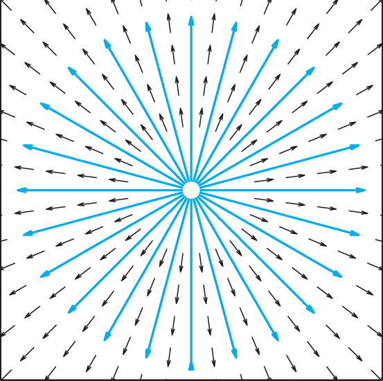
$x (t) = c_{1} v_{1} e^{λ t} + c_{2} v_{2} e^{λ t} = e^{λ t} (c_{1} v_{1} + c_{2} v_{2}) = e^{λ t} [\begin{array}{r} c_{1} \\ c_{2} \end{array}] .$

Either way, our solution in Eq. (25) shows that x(t) is always a positive scalar multiple of the fixed vector ${[\begin{array}{l} c_{1} & c_{2} \end{array}]}^{T} .$ Thus apart from the case $c_{1} = c_{2} = 0,$ the trajectories of the system (1) are half-lines, or rays, emanating from the origin and (because $λ > 0$ ) flowing away from it. As noted above, the origin in this case represents a proper node, because no two pairs of “opposite” solution curves are tangent to the same straight line through the origin. Moreover the origin is also a source (rather than a sink), and so in this case we call the origin a proper nodal source. Figure 7.4.6 shows the “exploding star” pattern characteristic of such points.

Example 6

The solution curves in Fig.7.4.6 correspond to the case where the matrix A is given by Eq. (22) with $λ = 2$ :

$A = [\begin{array}{r} 2 & 0 \\ 0 & 2 \end{array}] .$ (26)

FIGURE 7.4.6.

Solution curves $x (t) = e^{λ t} [\begin{array}{l} c_{1} \\ c_{2} \end{array}]$ for the system $x ′ = Ax$ when A has one repeated positive eigenvalue and two linearly independent eigenvectors.

Equation (25) then gives the general solution of the system $x ′ = A x$ as

$x (t) = e^{2 t} [\begin{array}{c} c_{1} \\ c_{2} \end{array}],$ (27)

or, in scalar form,

$\begin{array}{rcl} x_{1} (t) & = & c_{1} e^{2 t}, \\ x_{2} (t) & = & c_{2} e^{2 t} . \end{array}$

Our gallery Fig. 7.4.16 shows a more complete set of solution curves, together with a direction field, for the system $x ′ = A x$ with A given by Eq. (26).

Without two independent eigenvectors: The remaining possibility is that the matrix A has a repeated positive eigenvalue yet fails to have two linearly independent eigenvectors. In this event the general solution of the system $x ′ = A x$ is given by Eq. (7) above:

$x (t) = c_{1} v_{1} e^{λ t} + c_{2} (v_{1} t + v_{2}) e^{λ t} .$ (7)

Here $v_{1}$ is an eigenvector of the matrix A associated with the repeated eigenvalue $λ$ and $v_{2}$ is a (nonzero) “generalized eigenvector” that will be described more fully in Section 7.6. To analyze this trajectory, we first distribute the factor $e^{λ t}$ in Eq. (7), leading to

$x (t) = c_{1} v_{1} e^{λ t} + c_{2} (v_{1} t e^{λ t} + v_{2} e^{λ t}) .$ (28)

Our assumption that $λ > 0$ implies that both $e^{λ t}$ and ${t e}^{λ t}$ approach zero as $t \to - \infty,$ and so by Eq. (28) the solution x(t) approaches the origin as $t \to - \infty .$ Except for the trivial solution given by $c_{1} = c_{2} = 0,$ all trajectories given by Eq. (7) “emanate” from the origin as t increases.

The direction of flow of these curves can be understood from the tangent vector $x ′ (t) .$ Rewriting Eq. (28) as

$x (t) = e^{λ t} [c_{1} v_{1} + c_{2} (v_{1} t + v_{2})]$

and applying the product rule for vector-valued functions gives

$\begin{array}{rcl} x^{′} (t) & = & e^{λ t} c_{2} v_{2} + λ e^{λ t} [c_{1} v_{1} + c_{2} (v_{1} t + v_{2})] \\ = & e^{λ t} (c_{2} v_{1} + λ c_{1} v_{1} + λ c_{2} v_{1} t + λ c_{2} v_{2}) . \end{array}$ (29)

For $t \neq 0,$ we can factor out t in Eq. (29) and rearrange terms to get

$x^{′} (t) = t e^{λ t} [λ c_{2} v_{1} + \frac{1}{t} (λ c_{1} v_{1} + λ c_{2} v_{2} + c_{2} v_{1})] .$ (30)

Equation (30) shows that for $t \neq 0,$ the tangent vector $x ′ (t)$ is a nonzero scalar multiple of the vector $λ c_{2} v_{1} + \frac{1}{t} (λ c_{1} v_{1} + λ c_{2} v_{2} + c_{2} v_{1}),$ which, if $c_{2} \neq 0,$ approaches the fixed nonzero multiple $λ c_{2} v_{1}$ of the eigenvector $v_{1}$ as $t \to + \infty$ or as $t \to - \infty .$ In this case it follows that as t gets larger and larger numerically (in either direction), the tangent line to the solution curve at the point x(t)—since it is parallel to the tangent vector $x ′ (t)$ which approaches $λ c_{2} v_{1}$ —becomes more and more nearly parallel to the eigenvector $v_{1} .$ In short, we might say that as t increases numerically, the point x(t) on the solution curve moves in a direction that is more and more nearly parallel to the vector $v_{1},$ or still more briefly, that near x(t) the solution curve itself is virtually parallel to $v_{1}$ .

We conclude that if $c_{2} \neq 0,$ then as $t \to - \infty$ the point x(t) approaches the origin along the solution curve which is tangent there to the vector $v_{1} .$ But as $t \to + \infty$ and the point x(t) recedes farther and farther from the origin, the tangent line to the trajectory at this point tends to differ (in direction) less and less from the (moving) line through x(t) that is parallel to the (fixed) vector $v_{1} .$ Speaking loosely but suggestively, we might therefore say that at points sufficiently far from the origin, all trajectories are essentially parallel to the single vector $v_{1}$ .

If instead $c_{2} = 0,$ then our solution (7) becomes

$x (t) = c_{1} v_{1} e^{λ t},$ (31)

and thus runs along the line $l_{1}$ passing through the origin and parallel to the eigenvector $v_{1} .$ Because $λ > 0, x (t)$ flows away from the origin as t increases; the flow is in the direction of $v_{1}$ if $c_{1} > 0,$ and opposite $v_{1}$ if $c_{1} < 0$ .

We can further see the influence of the coefficient $c_{2}$ by writing Eq. (7) in yet a different way:

$x (t) = c_{1} v_{1} e^{λ t} + c_{2} (v_{1} t + v_{2}) e^{λ t} = (c_{1} + c_{2} t) v_{1} e^{λ t} + c_{2} v_{2} e^{λ t} .$ (32)

It follows from Eq. (32) that if $c_{2} \neq 0,$ then the solution curve x(t) does not cross the line $l_{1} .$ Indeed, if $c_{2} > 0,$ then Eq. (32) shows that for all t, the solution curve x(t) lies on the same side of $l_{1}$ as $v_{2},$ whereas if $c_{2} < 0,$ then x(t) lies on the opposite side of $l_{1}$ .

To see the overall picture, then, suppose for example that the coefficient $c_{2} > 0 .$ Starting from a large negative value of t, Eq. (30) shows that as t increases, the direction in which the solution curve x(t) initially proceeds from the origin is roughly that of the vector ${t e}^{λ t} λ c_{2} v_{1} .$ Since the scalar ${t e}^{λ t} λ c_{2}$ is negative (because $t < 0$ and $λ c_{2} > 0$ ), the direction of the trajectory is opposite that of $v_{1} .$ For large positive values of t, on the other hand, the scalar ${t e}^{λ t} λ c_{2}$ is positive, and so x(t) flows in nearly the same direction as $v_{1} .$ Thus, as t increases from $- \infty$ to $+ \infty,$ the solution curve leaves the origin flowing in the direction opposite $v_{1},$ makes a “U-turn” as it moves away from the origin, and ultimately flows in the direction of $v_{1}$ .

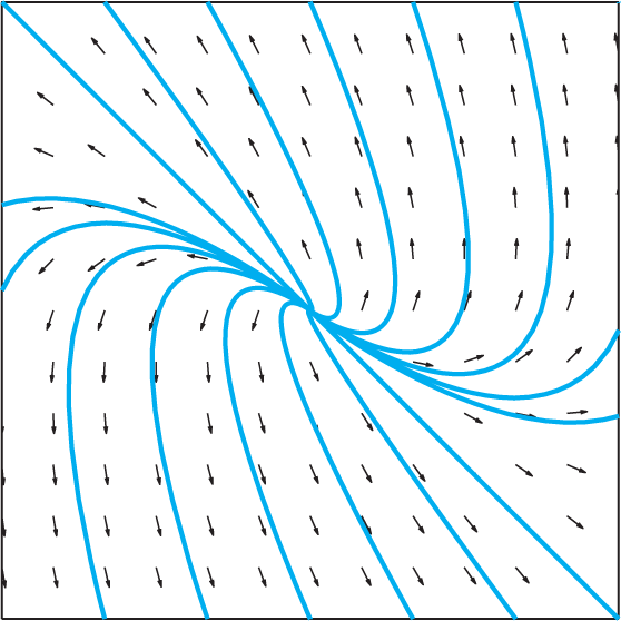
Because all nonzero trajectories are tangent at the origin to the line $l_{1},$ the origin represents an improper nodal source. Figure 7.4.7 illustrates typical solution curves given by $x (t) = c_{1} v_{1} e^{λ t} + c_{2} (v_{1} t + v_{2}) e^{λ t}$ for the system $x ′ = A x$ when A has a repeated eigenvalue but does not have two linearly independent eigenvectors.

FIGURE 7.4.7.

Solution curves $x (t) = c_{1} v_{1} e^{λ t} + c_{2} (v_{1} t + v_{2}) e^{λ t}$ for the system $x ′ = Ax$ when A has one repeated positive eigenvalue $λ$ with associated eigenvector $v_{1}$ and “generalized eigenvector” $v_{2}$ .

Example 7

The solution curves in Fig. 7.4.7 correspond to the choice

$A = [\begin{array}{r} 1 & - 3 \\ 3 & 7 \end{array}]$ (33)

in the system $x ′ = A x .$ In Examples 2 and 3 of Section 7.6 we will see that A has the repeated eigenvalue $λ = 4$ with associated eigenvector and generalized eigenvector given by

$\begin{array}{l} v_{1} = [\begin{array}{r} - 3 \\ 3 \end{array}] & and & v_{2} = [\begin{array}{r} 1 \\ 0 \end{array}], \end{array}$ (34)

respectively. According to Eq. (7) the resulting general solution is

$x (t) = c_{1} [\begin{array}{r} - 3 \\ 3 \end{array}] e^{4 t} + c_{2} [\begin{array}{c} - 3 t + 1 \\ 3 t \end{array}] e^{4 t},$ (35)

or, in scalar form,

$\begin{array}{rcl} x_{1} (t) & = & (- 3 c_{2} t - 3 c_{1} + c_{2}) e^{4 t}, \\ x_{2} (t) & = & (3 c_{2} t + 3 c_{1}) e^{4 t} . \end{array}$

Our gallery Fig. 7.4.16 shows a more complete set of solution curves, together with a direction field, for the system $x ′ = A x$ with A given by Eq. (33).

Repeated Negative Eigenvalue: Once again the principle of time reversal shows that the solutions x(t) of the system $x ′ = A x$ are identical to those of $x ′ = - A x$ with t replaced by $- t$ ; hence these two systems share the same trajectories while flowing in opposite directions. Further, if the matrix A has the repeated negative eigenvalue $λ,$ then the matrix $- A$ has the repeated positive eigenvalue $- λ$ (Problem 31 again). Therefore, to construct phase portraits for the system $x ′ = A x$ when A has a repeated negative eigenvalue, we simply reverse the directions of the trajectories in the phase portraits corresponding to a repeated positive eigenvalue. These portraits are illustrated in Figs. 7.4.8 and 7.4.9. In Fig. 7.4.8 the origin represents a proper nodal sink, whereas in Fig. 7.4.9 it represents an improper nodal sink.

FIGURE 7.4.8.

Solution curves $x (t) = e^{λ t} [\begin{array}{l} c_{1} \\ c_{2} \end{array}]$ for the system $x ′ = Ax$ when A has one repeated negative eigenvalue $λ$ and two linearly independent eigenvectors.

FIGURE 7.4.9.

Solution curves $x (t) = c_{1} v_{1} e^{λ t} + c_{2} (v_{1} t + v_{2}) e^{λ t}$ for the system $x ′ = Ax$ when A has one repeated negative eigenvalue $λ$ with associated eigenvector $v_{1}$ and “generalized eigenvector” $v_{2}$ .

Example 8

The solution curves in Fig. 7.4.8 correspond to the choice

$A = - [\begin{array}{r} 2 & 0 \\ 0 & 2 \end{array}] = [\begin{array}{r} - 2 & 0 \\ 0 & - 2 \end{array}]$ (36)

in the system $x ′ = A x$ ; thus A is the negative of the matrix in Example 6. We can solve this system by applying the principle of time reversal to the solution found in Eq. (27): Replacing t with $- t$ in the right-hand side of Eq. (27) leads to

$x (t) = e^{- 2 t} [\begin{array}{r} c_{1} \\ c_{2} \end{array}],$ (37)

or, in scalar form,

$\begin{array}{rcl} x_{1} (t) & = & c_{1} e^{- 2 t}, \\ x_{1} (t) & = & c_{2} e^{- 2 t} . \end{array}$

Alternatively, because A is given by Eq. (22) with $λ = - 2$ , Eq. (25) leads directly to the solution in Eq. (37). Our gallery Fig. 7.4.16 shows a more complete set of solution curves, together with a direction field, for the system $x ′ = A x$ with A given by Eq. (36).

Example 9

The solution curves in Fig. 7.4.9 correspond to the choice

$A = - [\begin{array}{r} 1 & - 3 \\ 3 & 7 \end{array}] = [\begin{array}{r} - 1 & 3 \\ - 3 & - 7 \end{array}]$ (38)

in the system $x ′ = A x .$ Thus A is the negative of the matrix in Example 7, and once again we can apply the principle of time reversal to the solution found in Eq. (35): Replacing t with $- t$ in the right-hand side of Eq. (35) yields

$x (t) = c_{1} [\begin{array}{r} - 3 \\ 3 \end{array}] e^{- 4 t} + c_{2} [\begin{array}{c} 3 t + 1 \\ - 3 t \end{array}] e^{- 4 t} .$ (39)

We could also arrive at an equivalent form of the solution in Eq. (39) in the following way. You can verify that A has the repeated eigenvalue $λ = - 2$ with eigenvector $v_{1}$ given by Eq. (34), that is,

$v_{1} = [\begin{array}{r} - 3 \\ 3 \end{array}] .$

However, as the methods of Section 7.6 will show, a generalized eigenvector $v_{2}$ associated with $v_{1}$ is now given by

$v_{2} = - [\begin{array}{r} 1 \\ 0 \end{array}] = [\begin{array}{r} - 1 \\ 0 \end{array}];$

that is, $v_{2}$ is the negative of the generalized eigenvector in Eq. (34). Equation (7) then gives the general solution of the system $x ′ = A x$ as

$x (t) = c_{1} [\begin{array}{r} - 3 \\ 3 \end{array}] e^{- 4 t} + c_{2} [\begin{array}{c} - 3 t - 1 \\ 3 t \end{array}] e^{- 4 t},$ (40)

or, in scalar form,

$\begin{array}{rcl} x_{1} (t) & = & (- 3 c_{2} t - 3 c_{1} - c_{2}) e^{- 4 t}, \\ x_{2} (t) & = & (3 c_{2} t + 3 c_{1}) e^{- 4 t} . \end{array}$

Note that replacing $c_{2}$ with $- c_{2}$ in the solution (39) yields the solution (40), thus confirming that the two solutions are indeed equivalent. Our gallery Fig. 7.4.16 shows a more complete set of solution curves, together with a direction field, for the system $x ′ = A x$ with A given by Eq. (38).

The Special Case of a Repeated Zero Eigenvalue

Repeated Zero Eigenvalue: Once again the matrix A may or may not have two linearly independent eigenvectors associated with the repeated eigenvalue $λ = 0 .$ If it does, then (using Problem 33 once more)we conclude that every nonzero vector is an eigenvector of A, that is, that $A v = 0 \cdot v = 0$ for all two-dimensional vectors v. It follows that A is the zero matrix of order two, that is,

$A = [\begin{array}{r} 0 & 0 \\ 0 & 0 \end{array}] .$

Therefore the system $x ′ = A x$ reduces to $x_{1}^{′} (t) = x_{2}^{′} (t) = 0,$ which is to say that $x_{1} (t)$ and $x_{2} (t)$ are each constant functions. Thus the general solution of $x ′ = A x$ is simply

$x (t) = [\begin{array}{l} c_{1} \\ c_{2} \end{array}],$ (41)

where $c_{1}$ and $c_{2}$ are arbitrary constants, and the “trajectories” given by Eq. (41) are simply the fixed points $(c_{1}, c_{2})$ in the phase plane.

If instead A does not have two linearly independent eigenvectors associated with $λ = 0,$ then the general solution of the system $x ′ = A x$ is given by Eq. (7) with $λ = 0$ :

$x (t) = c_{1} v_{1} + c_{2} (v_{1} t + v_{2}) = (c_{1} v_{1} + c_{2} v_{2}) + c_{2} v_{2} t .$ (42)

Once again $v_{1}$ denotes an eigenvector of the matrix A associated with the repeated eigenvalue $λ = 0$ and $v_{2}$ denotes a corresponding nonzero “generalized eigenvector.” If $c_{2} \neq 0,$ then the trajectories given by Eq. (42) are lines parallel to the eigenvector $v_{1}$ and “starting” at the point $c_{1} v_{1} + c_{2} v_{2}$ (when $t = 0$ ). When $c_{2} > 0$ the trajectory proceeds in the same direction as $v_{1},$ whereas when $c_{2} < 0$ the solution curve flows in the direction opposite $v_{1} .$ Once again the lines $l_{1}$ and $l_{2}$ passing through the origin and parallel to the vectors $v_{1}$ and $v_{2},$ respectively, divide the plane into “quadrants” corresponding to the signs of the coefficients $c_{1}$ and $c_{2}$ . The particular quadrant in which the “starting point” $c_{1} v_{1} + c_{2} v_{2}$ of the trajectory falls is determined by the signs of $c_{1}$ and $c_{2} .$ Finally, if $c_{2} = 0$ , then Eq. (42) gives $x (t) \equiv c_{1} v_{1}$ for all t, which means that each fixed point $c_{1} v_{1}$ along the line $l_{1}$ corresponds to a solution curve. (Thus the line $l_{1}$ could be thought of as a median strip dividing two opposing lanes of traffic.) Figure 7.4.10 illustrates typical solution curves corresponding to nonzero values of the coefficients $c_{1}$ and $c_{2}$ .

FIGURE 7.4.10.

Solution curves $x (t) = (c_{1} v_{1} + c_{2} v_{2}) + c_{2} v_{1} t$ for the system $x ′ = Ax$ when A has a repeated zero eigenvalue with associated eigenvector $v_{1}$ and “generalized eigenvector” $v_{2} .$ The emphasized point on each solution curve corresponds to $t = 0$ .

Example 10

The solution curves in Fig. 7.4.10 correspond to the choice

$A = [\begin{array}{r} 2 & 4 \\ - 1 & - 2 \end{array}]$ (43)

in the system $x ′ = A x .$ You can verify that $v_{1} = {[\begin{array}{l} 2 & - 1 \end{array}]}^{T}$ is an eigenvector of A associated with the repeated eigenvalue $λ = 0 .$ Further, using the methods of Section 7.6 we can show that $v_{2} = {[\begin{array}{r} 1 & 0 \end{array}]}^{T}$ is a corresponding “generalized eigenvector” of A. According to Eq. (42) the general solution of the system $x ′ = A x$ is therefore

$x (t) = c_{1} [\begin{array}{r} 2 \\ - 1 \end{array}] + c_{2} ([\begin{array}{r} 2 \\ - 1 \end{array}] t + [\begin{array}{r} 1 \\ 0 \end{array}]),$ (44)

or, in scalar form,

$\begin{array}{rcl} x_{1} (t) & = & 2 c_{1} + (2 t + 1) c_{2}, \\ x_{2} (t) & = & - c_{1} - t c_{2} . \end{array}$

Our gallery Fig.7.4.16 shows a more complete set of solution curves, together with a direction field, for the system $x ′ = A x$ with A given by Eq. (43).

Complex Conjugate Eigenvalues and Eigenvectors

We turn now to the situation in which the eigenvalues $λ_{1}$ and $λ_{2}$ of the matrix A are complex conjugate. As we noted at the beginning of this section, the general solution of the system $x ′ = A x$ is given by Eq. (5):

$x (t) = c_{1} e^{p t} (a \cos q t - b \sin q t) + c_{2} e^{p t} (b \cos q t + a \sin q t) .$ (5)

Here the vectors a and b are the real and imaginary parts, respectively, of a (complex-valued) eigenvector of A associated with the eigenvalue $λ_{1} = p + i q .$ We will divide the case of complex conjugate eigenvalues according to whether the real part p of $λ_{1}$ and $λ_{2}$ is zero, positive, or negative:

Pure imaginary ( $λ_{1}, λ_{2} = \pm i q$ with $q \neq 0$ )
Complex with negative real part ( $λ_{1}, λ_{2} = p \pm i q$ with $p < 0$ and $q \neq 0$ )
Complex with positive real part ( $λ_{1}, λ_{2} = p \pm i q$ with $p > 0$ and $q \neq 0$ )

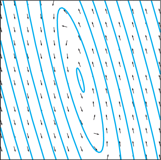
Pure Imaginary Eigenvalues: Centers and Elliptical Orbits

Pure Imaginary Eigenvalues: Centers and Elliptical Orbits Here we assume that the eigenvalues of the matrix A are given by $λ_{1}$ $λ_{2} = \pm i q$ with $q \neq 0 .$ Taking $p = 0$ in Eq. (5) gives the general solution

$x (t) = c_{1} (a \cos q t - b \sin q t) + c_{2} (b \cos q t + a \sin q t) .$ (45)

for the system $x ′ = A x .$ Rather than directly analyze the trajectories given by Eq. (45), as we have done in the previous cases, we begin instead with an example that will shed light on the nature of these solution curves.

Example 11

Solve the initial value problem

$\begin{array}{l} x^{′} = [\begin{array}{r} 6 & - 17 \\ 8 & - 16 \end{array}] x, & x (0) = [\begin{array}{r} 4 \\ 2 \end{array}] . \end{array}$ (46)

Solution

The coefficient matrix

$A = [\begin{array}{r} 6 & - 17 \\ 8 & - 6 \end{array}]$ (47)

has characteristic equation

$| A - λ I | = [\begin{array}{c} 6 - λ & - 17 \\ 8 & - 6 - λ \end{array}] = λ^{2} + 100 = 0,$

and hence has the complex conjugate eigenvalues $λ_{1}, λ_{2} = \pm 10 i .$ If $v = {[\begin{array}{l} a & b \end{array}]}^{T}$ is an eigenvector associated with $λ = 10 i,$ then the eigenvector equation $(A - λ I) v = 0$ yields

$[A - 10 i \cdot I] v = [\begin{array}{c} 6 - 10 i & - 17 \\ 8 & - 6 - 10 i \end{array}] [\begin{array}{c} a \\ b \end{array}] = [\begin{array}{c} 0 \\ 0 \end{array}] .$

Upon division of the second row by 2, this gives the two scalar equations

$\begin{array}{rcrcl} (6 - 10 i) a & - & 17 b & = & 0, \\ 4 a & - & (3 + 5 i) b & = & 0, \end{array}$ (48)

each of which is satisfied by $a = 3 + 5 i$ and $b = 4 .$ Thus the desired eigenvector is $v = {[\begin{array}{l} 3 & + & 5 i & 4 \end{array}]}^{T},$ with real and imaginary parts

$\begin{array}{l} a = [\begin{array}{c} 3 \\ 4 \end{array}] & and & b = [\begin{array}{c} 5 \\ 0 \end{array}], \end{array}$ (49)

respectively. Taking $q = 10$ in Eq. (45) therefore gives the general solution of the system $x ′ = A x$ :

$\begin{array}{rcl} x (t) & = & c_{1} ([\begin{array}{c} 3 \\ 4 \end{array}] \cos 10 t - [\begin{array}{c} 5 \\ 0 \end{array}] \sin 10 t) + ([\begin{array}{c} 5 \\ 0 \end{array}] \cos 10 t + [\begin{array}{c} 3 \\ 4 \end{array}] \sin 10 t) \\ = & [\begin{array}{c} c_{1} (3 \cos 10 t - 5 \sin 10 t) + c_{2} (5 \cos 10 t + 3 \sin 10 t) \\ 4 c_{1} \cos 10 t + 4 c_{2} \sin 10 t \end{array}] . \end{array}$ (50)

To solve the given initial value problem it remains only to determine values of the coefficients $c_{1}$ and $c_{2} .$ The initial condition $x (0) = {[\begin{array}{l} 4 & 2 \end{array}]}^{T}$ readily yields $c_{1} = c_{2} = \frac{1}{2},$ and with these values Eq. (50) becomes (in scalar form)

$\begin{array}{rcl} x_{1} (t) & = & 4 \cos 10 t - \sin 10 t, \\ x_{2} (t) & = & 2 \cos 10 t + 2 \sin 10 t . \end{array}$ (51)

Figure 7.4.11 shows the trajectory given by Eq. (51) together with the initial point (4, 2).

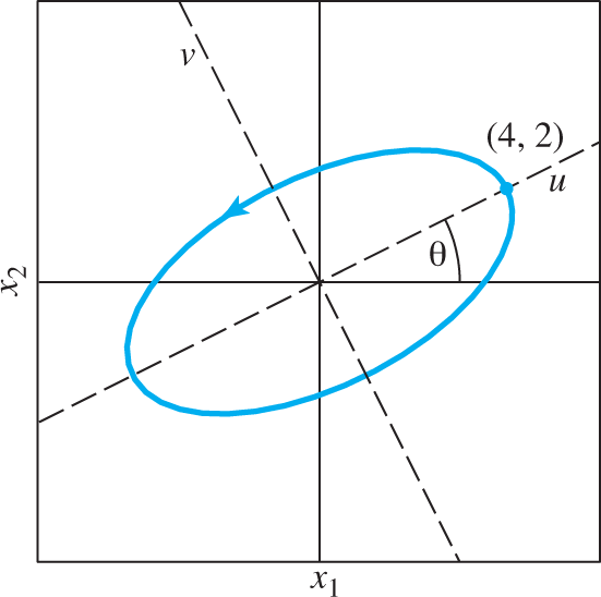
FIGURE 7.4.11.

Solution curve $x_{1} (t) = 4 \cos 10 t - \sin 10 t, x_{2} (t) = 2 \cos 10 t + 2 \sin 10 t$ for the initial value problem in Eq. (46).

This solution curve appears to be an ellipse rotated counterclockwise by the angle $θ = \arctan \frac{2}{4} \approx 0.4636.$ We can verify this by finding the equations of the solution curve relative to the rotated u- and v-axes shown in Fig. 7.4.11. By a standard formula from analytic geometry, these new equations are given by

$\begin{array}{rcl} u & = & x_{1} \cos θ + x_{2} \sin θ = \frac{2}{\sqrt{5}} x_{1} + \frac{1}{\sqrt{5}} x_{2}, \\ v & = & - x_{1} \sin θ + x_{2} \cos θ = - \frac{1}{\sqrt{5}} x_{1} + \frac{2}{\sqrt{5}} x_{2} . \end{array}$ (52)

In Problem 34 we ask you to substitute the expressions for $x_{1}$ and $x_{2}$ from Eq. (51) into Eq. (52), leading (after simplification) to

$\begin{array}{l} u = 2 \sqrt{5} \cos 10 t, & v = \sqrt{5} \sin 10 t . \end{array}$ (53)

Equation (53) not only confirms that the solution curve in Eq. (51) is indeed an ellipse rotated by the angle $θ,$ but it also shows that the lengths of the semi-major and semi-minor axes of the ellipse are $2 \sqrt{5}$ and $\sqrt{5}$ , respectively.

Furthermore, we can demonstrate that any choice of initial point (apart from the origin) leads to a solution curve that is an ellipse rotated by the same angle $θ$ and “concentric” (in an obvious sense) with the trajectory in Fig.7.4.11 (see Problems 35–37). All these concentric rotated ellipses are centered at the origin (0, 0), which is therefore called a center for the system $x ′ = A x$ whose coefficient matrix A has pure imaginary eigenvalues. Our gallery Fig.7.4.16 shows a more complete set of solution curves, together with a direction field, for the system $x ′ = A x$ with A given by Eq. (47).

Further investigation: Geometric significance of the eigenvector. Our general solution in Eq. (50) was based upon the vectors a and b in Eq. (49), that is, the real and imaginary parts of the complex eigenvector $v = {[\begin{array}{l} 3 + 5 i & 4 \end{array}]}^{T}$ of the matrix A. We might therefore expect a and b to have some clear geometric connection to the solution curve in Fig. 7.4.11. For example, we might guess that a and b would be parallel to the major and minor axes of the elliptical trajectory. However, it is clear from Fig. 7.4.12—which shows the vectors a and b together with the solution curve given by Eq. (51)—that this is not the case. Do the eigenvectors of A, then, play any geometric role in the phase portrait of the system $x ′ = A x$ ?

FIGURE 7.4.12.

Solution curve for the initial value problem in Eq. (46) showing the vectors a, b, $\tilde{a},$ and $\tilde{b}$ .

The (affirmative) answer lies in the fact that any nonzero real or complex multiple of a complex eigenvector of the matrix A is still an eigenvector of A associated with that eigenvalue. Perhaps, then, if we multiply the eigenvector $v = {[\begin{array}{l} 3 + 5 i & 4 \end{array}]}^{T}$ by a suitable nonzero complex constant z, the resulting eigenvector $\tilde{v}$ will have real and imaginary parts $\tilde{a}$ and $\tilde{b}$ that can be readily identified with geometric features of the ellipse. To this end, let us multiply $v$ by the complex scalar $z = \frac{1}{2} (1 + i) .$ (The reason for this particular choice will become clear shortly.)The resulting new complex eigenvector $\tilde{v}$ of the matrix A is,

$\tilde{v} = z \cdot v = \frac{1}{2} (1 + i) \cdot [\begin{array}{c} 3 + 5 i \\ 4 \end{array}] = [\begin{array}{r} - 1 + 4 i \\ 2 + 2 i \end{array}],$

and has real and imaginary parts

$\begin{array}{l} \tilde{a} = [\begin{array}{r} - 1 \\ 2 \end{array}] & and & \tilde{b} = [\begin{array}{c} 4 \\ 2 \end{array}] . \end{array}$

It is clear that the vector $\tilde{b}$ is parallel to the major axis of our elliptical trajectory. Further, you can easily check that $\tilde{a} \cdot \tilde{b} = 0,$ which means that $\tilde{a}$ is perpendicular to $\tilde{b},$ and hence is parallel to the minor axis of the ellipse, as Fig. 7.4.12 illustrates. Moreover, the length of $\tilde{b}$ is twice that of $\tilde{a},$ reflecting the fact that the lengths of the major and minor axes of the ellipse are in this same ratio. Thus for a matrix A with pure imaginary eigenvalues, the complex eigenvector of A used in the general solution (45)—if suitably chosen—is indeed of great significance to the geometry of the elliptical solution curves of the system $x ′ = A x$ .

How was the value $\frac{1}{2} (1 + i)$ chosen for the scalar z? In order that the real and imaginary parts $\tilde{a}$ and $\tilde{b}$ of $\tilde{v} = z \cdot v$ be parallel to the axes of the ellipse, at a minimum $\tilde{a}$ and $\tilde{b}$ must be perpendicular to each other. In Problem 38 we ask you to show that this condition is satisfied if and only if z is of the form $r (1 \pm i),$ where r is a nonzero real number, and that if z is chosen in this way, then $\tilde{a}$ and $\tilde{b}$ are in fact parallel to the axes of the ellipse. The value $r = \frac{1}{2}$ then aligns the lengths of $\tilde{a}$ and $\tilde{b}$ with those of the semi-minor and -major axes of the elliptical trajectory. More generally, we can show that given any eigenvector v of a matrix A with pure imaginary eigenvalues, there exists a constant z such that the real and imaginary parts $\tilde{a}$ and $\tilde{b}$ of the eigenvector $\tilde{v} = z \cdot v$ are parallel to the axes of the (elliptical) trajectories of the system $x ′ = A x$ .

Further investigation: Direction of flow. Figs. 7.4.11 and 7.4.12 suggest that the solution curve in Eq. (51) flows in a counterclockwise direction with increasing t. However, you can check that the matrix

$- A = [\begin{array}{r} - 6 & 17 \\ - 8 & 6 \end{array}]$

has the same eigenvalues and eigenvectors as the matrix A in Eq. (47) itself, and yet (by the principle of time reversal) the trajectories of the system $x ′ = - A x$ are identical to those of $x ′ = A x$ while flowing in the opposite direction, that is, clockwise. Clearly, mere knowledge of the eigenvalues and eigenvectors of the matrix A is not sufficient to predict the direction of flow of the elliptical trajectories of the system $x ′ = A x$ as t increases. How then can we determine this direction of flow?

One simple approach is to use the tangent vector $x ′$ to monitor the direction in which the solution curves flow as they cross the positive $x_{1}$ -axis. If s is any positive number (so that the point (s, 0) lies on the positive $x_{1}$ -axis), and if the matrix A is given by

$A = [\begin{array}{l} a & b \\ c & d \end{array}],$

then any trajectory for the system $x ′ = A x$ passing through (s, 0) satisfies

$x^{′} = A x = [\begin{array}{l} a & b \\ c & d \end{array}] [\begin{array}{l} s \\ 0 \end{array}] = [\begin{array}{l} a s \\ c s \end{array}] = s [\begin{array}{l} a \\ c \end{array}]$

at the point (s, 0). Therefore, at this point the direction of flow of the solution curve is a positive scalar multiple of the vector ${[\begin{array}{r} a & c \end{array}]}^{T} .$ Since c cannot be zero (see Problem 39), this vector either points “upward” into the first quadrant of the phase plane (if $c > 0$ ), or “downward” into the fourth quadrant (if $c < 0$ ). If upward, then the flow of the solution curve is counterclockwise; if downward, then clockwise. For the matrix A in Eq. (47), the vector ${[\begin{array}{r} a & c \end{array}]}^{T} = {[\begin{array}{r} 6 & 8 \end{array}]}^{T}$ points into the first quadrant because $c = 8 > 0,$ thus indicating a counterclockwise direction of flow (as Figs. 7.4.11 and 7.4.12 suggest).

Complex Eigenvalues: Spiral Sinks and Sources

Complex Eigenvalues with Negative Real Part: Now we assume that the eigenvalues of the matrix A are given by $λ_{1}, λ_{2} = p \pm i q$ with $q \neq 0$ and $p < 0$ . In this case the general solution of the system $x ′ = A x$ is given directly by Eq. (5):

$x (t) = c_{1} e^{p t} (a \cos q t - b \sin q t) + c_{2} e^{p t} (b \cos q t + a \sin q t),$ (5)

where the vectors a and b have their usual meaning. Once again we begin with an example to gain an understanding of these solution curves.

Example 12

Solve the initial value problem

$x^{′} = [\begin{array}{r} 5 & - 17 \\ 8 & - 7 \end{array}] x, x (0) = [\begin{matrix} 4 \\ 2 \end{matrix}] .$ (54)

Solution

The coefficient matrix

$A = [\begin{array}{rr} 5 & - 17 \\ 8 & - 7 \end{array}]$ (55)

has characteristic equation

$| A - λ I | = | \begin{array}{cc} 5 - λ & - 17 \\ 8 & - 7 - λ \end{array} | = {(λ + 1)}^{2} + 100 = 0,$

and hence has the complex conjugate eigenvalues $λ_{1}, λ_{2} = - 1 \pm 10 i$ . If $v = {[\begin{array}{rr} a & b \end{array}]}^{T}$ is an eigenvector associated with $λ = - 1 + 10 i$ , then the eigenvector equation $(A - λ I) v = 0$ yields the same system (48) of equations found in Example 11:

$\begin{array}{r} (6 - 10 i) a & - & 17 b & = & 0, \\ 4 a & - & (3 + 5 i) b & = & 0. \end{array}$ (48)

As in Example 11, each of these equations is satisfied by $a = 3 + 5 i$ and $b = 4$ . Thus the desired eigenvector, associated with $λ_{1} = - 1 + 10 i$ , is once again $v = {[3 + 5 i 4]}^{T},$ with real and imaginary parts

$a = [\begin{array}{rr} 3 \\ 4 \end{array}] and b = [\begin{array}{rr} 5 \\ 0 \end{array}],$ (56)

respectively. Taking $p = - 1$ and $q = 10$ in Eq. (5) therefore gives the general solution of the system $x ′ = A x$ :

$\begin{aligned} x (t) & = & c_{1} e^{- t} ([\begin{array}{c} 3 \\ 4 \end{array}] \cos 10 t - [\begin{array}{c} 5 \\ 0 \end{array}] \sin 10 t) + c_{2} e^{- t} ([\begin{array}{c} 5 \\ 0 \end{array}] \cos 10 t + [\begin{array}{c} 3 \\ 4 \end{array}] \sin 10 t) \\ = & [\begin{array}{c} c_{1} e^{- t} (3 \cos 10 t - 5 \sin 10 t) + c_{2} e^{- t} (5 \cos 10 t + 3 \sin 10 t) \\ 4 c_{1} e^{- t} \cos 10 t + 4 c_{2} e^{- t} \sin 10 t \end{array}] . \end{aligned}$ (57)

The initial condition $x (0) = {[\begin{array}{l} 4 & 2 \end{array}]}^{T}$ gives $c_{1} = c_{2} = \frac{1}{2}$ once again, and with these values Eq. (57) becomes (in scalar form)

$\begin{array}{rcl} x_{1} (t) & = & e^{- t} (4 \cos 10 t - \sin 10 t), \\ x_{2} (t) & = & e^{- t} (2 \cos 10 t + 2 \sin 10 t) . \end{array}$ (58)

Figure 7.4.13 shows the trajectory given by Eq. (58) together with the initial point (4, 2). It is noteworthy to compare this spiral trajectory with the elliptical trajectory in Eq. (51). The equations for $x_{1} (t)$ and $x_{2} (t)$ in (58) are obtained by multiplying their counterparts in (51) by the common factor $e^{- t}$ , which is positive and decreasing with increasing t. Thus for positive values of t, the spiral trajectory is generated, so to speak, by standing at the origin and “reeling in” the point on the elliptical trajectory (51) as it is traced out. When t is negative, the picture is rather one of “casting away” the point on the ellipse farther out from the origin to create the corresponding point on the spiral.

FIGURE 7.4.13.

Solution curve $x_{1} (t) = e^{- t} (4 \cos 10 t - \sin 10 t), x_{2} (t) = e^{- t} (2 \cos 10 t + 2 \sin 10 t) .$ for the initial value problem in Eq. (54). The dashed and solid portions of the curve correspond to negative and positive values of `t`, respectively.

Our gallery Fig. 7.4.16 shows a more complete set of solution curves, together with a direction field, for the system $x ′ = A x$ with A given by Eq. (55). Because the solution curves all “spiral into” the origin, we call the origin in this a case a spiral sink.

Complex Eigenvalues with Positive Real Part: We conclude with the case where the eigenvalues of the matrix A are given by $λ_{1}, λ_{2} = p \pm i q$ with $q \neq 0$ and $p > 0$ . Just as in the preceding case, the general solution of the system $x ′ = A x$ is given by Eq. (5):

$x (t) = c_{1} e^{p t} (a \cos q t - b \sin q t) + c_{2} e^{p t} (b \cos q t + a \sin q t) .$ (5)

An example will illustrate the close relation between the cases $p > 0$ and $p < 0$ .

Example 13

Solve the initial value problem

$x^{′} = [\begin{array}{r} - 5 & 17 \\ - 8 & 7 \end{array}] x, x (0) = [\begin{array}{r} 4 \\ 2 \end{array}] .$ (59)

Solution

Although we could directly apply the eigenvalue/eigenvector method as in previous cases (see Problem 40), here it is more convenient to notice that the coefficient matrix

$A = [\begin{array}{r} - 5 & 17 \\ - 8 & 7 \end{array}]$ (60)

is the negative of the matrix in Eq. (55) used in Example 12. By the principle of time reversal, therefore, the solution of the initial value problem (59) is given by simply replacing t with $- t$ in the right-hand sides of the solution (58) of the initial value problem in that example:

$\begin{aligned} x_{1} (t) & = & e^{t} (4 \cos 10 t + \sin 10 t), \\ x_{2} (t) & = & e^{t} (2 \cos 10 t - 2 \sin 10 t) . \end{aligned}$ (61)

Figure 7.4.14 shows the trajectory given by Eq. (61) together with the initial point (4, 2). Our gallery Fig. 7.4.16 shows this solution curve together with a direction field for the system $x ′ = A x$ with A given by Eq. (60). Because the solution curve “spirals away from” the origin, we call the origin in this case a spiral source.

FIGURE 7.4.14.

Solution curve $x_{1} (t) = e^{t} (4 \cos 10 t + \sin 10 t), x_{2} (t) = e^{t} (2 \cos 10 t - 2 \sin 10 t)$ for the initial value problem in Eq. (59). The dashed and solid portions of the curve correspond to negative and positive values of `t`, respectively.

A 3-Dimensional Example

Figure 7.4.15 illustrates the space trajectories of solutions of the 3-dimensional system $x ′ = A x$ with constant coefficient matrix

$A = [\begin{array}{r} 4 & 10 & 0 \\ - 5 & - 6 & 0 \\ 0 & 0 & 1 \end{array}] .$ (62)

To portray the motion in space of a point x(t) moving on a trajectory of this system, we can regard this trajectory as a necklace string on which colored beads are placed to mark its successive positions at fixed increments of time (so the point is moving fastest where the spacing between beads is greatest). In order to aid the eye in following the moving point’s progress, the size of the beads decreases continuously with the passage of time and motion along the trajectory.

FIGURE 7.4.15.

Three-dimensional trajectories for the system $x ′ = A x$ with the matrix A given by Eq. (62).

The matrix A has the single real eigenvalue $- 1$ with the single (real) eigenvector ${[\begin{array}{rrr} 0 & 0 & 1 \end{array}]}^{T}$ and the complex conjugate eigenvalues $- 1 \pm 5 i$ . The negative real eigenvalue corresponds to trajectories that lie on the $x_{3}$ -axis and approach the origin as $t \to 0$ (as illustrated by the beads on the vertical axis of the figure). Thus the origin (0, 0, 0) is a sink that “attracts” all the trajectories of the system.

The complex conjugate eigenvalues with negative real part correspond to trajectories in the horizontal $x_{1} x_{2}$ -plane that spiral around the origin while approaching it. Any other trajectory—one which starts at a point lying neither on the z-axis nor in the $x_{1} x_{2}$ -plane—combines the preceding behaviors by spiraling around the surface of a cone while approaching the origin at its vertex.

Gallery of Typical Phase Portraits for the System $x ′ = A x :$ Nodes

FIGURE 7.4.16.

Gallery of typical phase plane portraits for the system $x ′ = A x$ .

Gallery of Typical Phase Portraits for the System $x ′ = A x :$ Saddles, Centers, Spirals, and Parallel Lines

7.4 Problems

For each of the systems in Problems 1 through 16 in Section 7.3, categorize the eigenvalues and eigenvectors of the coefficient matrix A according to Fig. 7.4.16 and sketch the phase portrait of the system by hand. Then use a computer system or graphing calculator to check your answer.

The phase portraits in Problems 17 through 28 correspond to linear systems of the form $x ′ = A x$ in which the matrix A has two linearly independent eigenvectors. Determine the nature of the eigenvalues and eigenvectors of each system. For example, you may discern that the system has pure imaginary eigenvalues, or that it has real eigenvalues of opposite sign; that an eigenvector associated with the positive eigenvalue is roughly ${[\begin{array}{r} 2 & - 1 \end{array}]}^{T},$ etc.

We can give a simpler description of the general solution

$x (t) = c_{1} [\begin{array}{r} - 1 \\ 6 \end{array}] e^{- 2 t} + c_{2} [\begin{array}{r} 1 \\ 1 \end{array}] e^{5 t}$ (9)

of the system

$x^{′} = [\begin{array}{rrr} 4 & 1 \\ 6 & - 1 \end{array}] x$

in Example 1 by introducing the oblique $u v$ -coordinate system indicated in Fig. 7.4.17, in which the u- and v-axes are determined by the eigenvectors $v_{1} = [\begin{array}{rrr} - 1 \\ 6 \end{array}]$ and $v_{2} = [\begin{array}{rrr} 1 \\ 1 \end{array}],$ respectively.

FIGURE 7.4.17.

The oblique uv-coordinate system determined by the eigenvectors $v_{1}$ and $v_{2}$ .

The $u v$ -coordinate functions u(t) and v(t) of the moving point x(t) are simply its distances from the origin measured in the directions parallel to $v_{1}$ and $v_{2}$ . It follows from (9) that a trajectory of the system is described by

$u (t) = u_{0} e^{- 2 t}, v (t) = v_{0} e^{5 t}$ (63)

where $u_{0} = u (0)$ and $v_{0} = v (0)$ . (a) Show that if $v_{0} = 0$ , then this trajectory lies on the u-axis, whereas if $u_{0} = 0$ , then it lies on the v-axis. (b) Show that if $u_{0}$ and $v_{0}$ are both nonzero, then a “Cartesian” equation of the parametric curve in Eq. (63) is given by $v = {C u}^{- 5/2}$ .
Use the chain rule for vector-valued functions to verify the principle of time reversal.

In Problems 31–33 A represents a $2 \times 2$ matrix.

Use the definitions of eigenvalue and eigenvector (Section 7.3) to prove that if $λ$ is an eigenvalue of A with associated eigenvector v, then $- λ$ is an eigenvalue of the matrix $- A$ with associated eigenvector v. Conclude that if A has positive eigenvalues $0 < λ_{2} < λ_{1}$ with associated eigenvectors $v_{1}$ and $v_{2}$ , then $- A$ has negative eigenvalues $- λ_{1} < - λ_{2} < 0$ with the same associated eigenvectors.
Show that the system $x ′ = A x$ has constant solutions other than $x (t) \equiv 0$ if and only if there exists a (constant) vector $x \neq 0$ with $A x = 0$ . (It is shown in linear algebra that such a vector x exists exactly when $det (A) = 0$ .)
(a) Show that if A has the repeated eigenvalue $λ$ with two linearly independent associated eigenvectors, then every nonzero vector v is an eigenvector of A. (Hint: Express v as a linear combination of the linearly independent eigenvectors and multiply both sides by A.) (b) Conclude that A must be given by Eq. (22). (Suggestion: In the equation $A v = λ v take v = {[\begin{array}{r} 1 & 0 \end{array}]}^{T} and v = {[\begin{array}{r} 0 & 1 \end{array}]}^{T} .)$
Verify Eq. (53) by substituting the expressions for $x_{1} (t)$ and $x_{2} (t)$ from Eq. (51) into Eq. (52) and simplifying.

Problems 35–37 show that all nontrivial solution curves of the system in Example 11 are ellipses rotated by the same angle as the trajectory in Fig. 7.4.11.

The system in Example 11 can be rewritten in scalar form as

$\begin{aligned} x_{1}^{′} & = & 6 x_{1} - 17 x_{2}, \\ x_{2}^{′} & = & 8 x_{1} - 6 x_{2}, \end{aligned}$

leading to the first-order differential equation

$\frac{d x_{2}}{d x_{1}} = \frac{d x_{2} / d t}{d x_{1} / d t} = \frac{8 x_{1} - 6 x_{2}}{6 x_{1} - 17 x_{2}},$

or, in differential form,

$(6 x_{2} - 8 x_{1}) d x_{1} + (6 x_{1} - 17 x_{2}) d x_{2} = 0.$

Verify that this equation is exact with general solution

$- 4 x_{1}^{2} + 6 x_{1} x_{2} - \frac{17}{2} x_{2}^{2} = k,$ (64)

where k is a constant.
In analytic geometry it is shown that the general quadratic equation

$A x_{1}^{2} + B x_{1} x_{2} + C x_{2}^{2} = k$ (65)

represents an ellipse centered at the origin if and only if $A k > 0$ and the discriminant $B^{2} - 4 A C < 0$ . Show that Eq. (64) satisfies these conditions if $k < 0$ , and thus conclude that all nondegenerate solution curves of the system in Example 11 are elliptical.
It can be further shown that Eq. (65) represents in general a conic section rotated by the angle $θ$ given by

$\tan 2 θ = \frac{B}{A - C} .$

Show that this formula applied to Eq. (64) leads to the angle $θ = \arctan \frac{2}{4}$ found in Example 11, and thus conclude that all elliptical solution curves of the system in Example 11 are rotated by the same angle $θ$ . (Suggestion: You may find useful the double-angle formula for the tangent function.)
Let $v = {[3 + 5 i 4]}^{T}$ be the complex eigenvector found in Example 11 and let z be a complex number. (a) Show that the real and imaginary parts $\tilde{a}$ and $\tilde{b}$ , respectively, of the vector $\tilde{v} = z \cdot v$ are perpendicular if and only if $z = r (1 \pm i)$ for some nonzero real number r. (b) Show that if this is the case, then $\tilde{a}$ and $\tilde{b}$ are parallel to the axes of the elliptical trajectory found in Example 11 (as Fig. 7.4.12 indicates).
Let A denote the $2 \times 2$ matrix

$A = [\begin{array}{r} a & b \\ c & d \end{array}] .$
1. Show that the characteristic equation of A (Eq. (3), Section 6.1) is given by
  
  $λ^{2} - (a + d) λ + (a d - b c) = 0 .$
2. Suppose that the eigenvalues of A are pure imaginary. Show that the trace $T (A) = a + d$ of A must be zero and that the determinant $D (A) = a d - b c$ must be positive. Conclude that $c \neq 0$ .
Use the eigenvalue/eigenvector method to confirm the solution in Eq. (61) of the initial value problem in Eq. (59).

7.4 Application Dynamic Phase Plane Graphics

Using computer systems we can “bring to life” the static gallery of phase portraits in Fig. 7.4.16 by allowing initial conditions, eigenvalues, and even eigenvectors to vary in “real time.” Such dynamic phase plane graphics afford additional insight into the relationship between the algebraic properties of the $2 \times 2$ matrix A and the phase plane portrait of the system $x ′ = A x$ .

For example, the basic linear system

$\begin{aligned} \frac{d x_{1}}{d t} & = & - x_{1}, \\ \frac{d x_{2}}{d t} & = & - k x_{2} & (k a nonzero constant), \end{aligned}$

has general solution

$x_{1} (t) = a e^{- t}, x_{2} (t) = b e^{- k t},$

where (a, b) is the initial point. If $a \neq 0$ , then we can write

$x_{2} = b e^{- k t} = \frac{b}{a^{k}} (a e^{- 1}) = c x_{1}^{k},$ (1)

where $c = b / a^{k}$ . A version of the Maple commands

with(plots):
createPlot := proc(k)
   soln := plot([exp(-t), exp(-k*t),
      t = -10..10], x = -5..5, y = -5..5):
return display(soln):
end proc:
Explore(createPlot(k),
   parameters = [k = -2.0..2.0])

produces Fig. 7.4.18, which allows the user to vary the parameter k continuously from $k = - 2$ to $k = 2$ , thus showing dynamically the changes in the solution curves (1) in response to changes in k.

FIGURE 7.4.18.

Interactive display of the solution curves in Eq. (1). Using the slider, the value of `k` can be varied continuously from $- 2$ to 2.

Figure 7.4.19 shows snapshots of the interactive display in Fig. 7.4.18 corresponding to the values $- 1, \frac{1}{2},$ and 2 for the parameter k. Based on this progression, how would you expect the solution curves in Eq. (1) to look when $k = 1$ ? Does Eq. (1) corroborate your guess?

FIGURE 7.4.19.

Snapshots of the interactive display in Fig. 7.4.18 with the initial conditions held fixed and the parameter `k` equal to $- 1, \frac{1}{2},$ and 2, respectively.

As another example, a version of the Mathematica commands

a = {{-5, 17}, {-8, 7}};
x[t_] := {x1[t], x2[t]};
Manipulate[
   soln = DSolve[{x′[t] == a.x[t],
      x[0] == pt[[1]]}, x[t], t];
   ParametricPlot[x[t]/.soln, {t, -3.5, 10},
      PlotRange -> 5],
   {{pt, {{4, 2}}}, Locator}]

was used to generate Fig. 7.4.20, which (like Figs. 7.4.13 and 7.4.14) shows the solution curve of the initial value problem

$x^{′} = [\begin{array}{rrr} - 5 & 17 \\ - 8 & 7 \end{array}] x, x (0) = [\begin{matrix} 4 \\ 2 \end{matrix}]$ (2)

from Example 13 of the preceding section. However, in Fig. 7.4.20 the initial condition (4, 2) is attached to a “locator point” which can be freely dragged to any desired position in the phase plane, with the corresponding solution curve being instantly redrawn—thus illustrating dynamically the effect of varying the initial conditions.

FIGURE 7.4.20.

Interactive display of the initial value problem in Eq. (2). As the “locator point” is dragged to different positions, the solution curve is immediately redrawn, showing the effect of changing the initial conditions.

FIGURE 7.4.21.

Interactive display of the initial value problem $x ′ = A x$ with A given by Eq. (3). Both the initial conditions and the value of the parameter `k` can be varied dynamically.

Finally, Fig. 7.4.21 shows a more sophisticated, yet perhaps more revealing, demonstration. As you can verify, the matrix

$A = \frac{1}{10} [\begin{array}{c} k + 9 & 3 - 3 k \\ 3 - 3 k & 9 k + 1 \end{array}]$ (3)

has the variable eigenvalues 1 and k but with fixed associated eigenvectors ${[\begin{array}{l} 3 & 1 \end{array}]}^{T}$ and ${[\begin{array}{l} 1 & - 3 \end{array}]}^{T},$ respectively. Figure 7.4.21, which was generated by a version of the Mathematica commands

a[k ] := (1/10){{k + 9, 3 - 3k}, {3 - 3k, 9k + 1}}
x[t ] := {x1[t], x2[t]}
Manipulate[
   soln[k ] = DSolve[{x′[t] == a[k].x[t],
      x[0] == #}, x[t], t]&/@pt;
   curve = ParametricPlot
      [Evaluate[x[t]/.soln[k]], {t, -10, 10},
      PlotRange -> 4], {k, -1, 1},
   {{pt, {{2, -1}, {1, 2}, {-1, -2}, {-2, 1}}},
   Locator}]

shows the phase portrait of the system $x ′ = A x$ with A given by Eq. (3). Not only are the initial conditions of the individual trajectories controlled independently by the “locator points,” but using the slider we can also vary the value of k continuously from $- 1$ to 1, with the solution curves being instantly redrawn. Thus for a fixed value of k we can experiment with changing initial conditions throughout the phase plane, or, conversely, we can hold the initial conditions fixed and observe the effect of changing the value of k.

As a further example of what such a display can reveal, Fig. 7.4.22 consists of a series of snapshots of Fig. 7.4.21 where the initial conditions are held fixed and k progresses through the specific values $- 1, - 0.25$ , 0, 0.5, 0.65, and 1. The result is a “video” showing stages in a transition from a saddle point with “hyperbolic” trajectories, to a pair of parallel lines, to an improper nodal source with “parabolic” trajectories, and finally to the exploding star pattern of a proper nodal source with straight-line trajectories. Perhaps these frames provide a new interpretation of the description “dynamical system” for a collection of interdependent differential equations.

FIGURE 7.4.22.

Snapshots of the interactive display in Fig. 7.4.21 with the initial conditions held fixed and the parameter `k` increasing from $- 1$ to 1.

..................Content has been hidden....................

You can't read the all page of ebook, please click here login for view all page.

Table of Contents for 7.4 A Gallery of Solution Curves of Linear Systems

Create new playlist

Sign In

Sign Up

Table of Contents for
7.4 A Gallery of Solution Curves of Linear Systems