
7.5 Second-Order Systems and Mechanical Applications*
In this section we apply the matrix methods of Sections 7.2 and 7.3 to investigate the oscillations of typical mass-and-spring systems having two or more degrees of freedom. Our examples are chosen to illustrate phenomena that are generally characteristic of complex mechanical systems.
Figure 7.5.1 shows three masses connected to each other and to two walls by the four indicated springs. We assume that the masses slide without friction and that each spring obeys Hooke’s law—its extension or compression x and force F of reaction are related by the formula F=−kx.
The first spring is stretched the distance x1
x1 ;The second spring is stretched the distance x2−x1
x2−x1 ;The third spring is stretched the distance x3−x2
x3−x2 ;The fourth spring is compressed the distance x3
x3 .
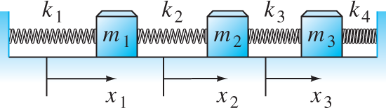
FIGURE 7.5.1.
Three spring-coupled masses.
Therefore, application of Newton’s law F=ma
Although we assumed in writing these equations that the displacements of themasses are all positive, they actually follow similarly from Hooke’s and Newton’s laws, whatever the signs of these displacements.
In terms of the displacement vector x=[x1x2x3]T,
and the stiffness matrix
the system in (1) takes the matrix form
![]()
The notation in Eqs. (1) through (4) generalizes in a natural way to the system of n spring-coupled masses shown in Fig. 7.5.2. We need only write
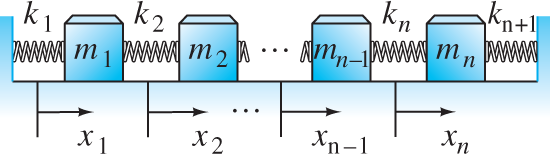
FIGURE 7.5.2.
A system of n spring-coupled masses.
and
for the mass and stiffness matrices in Eq. (4).
The diagonal matrix M is obviously nonsingular; to get its inverse M−1
![]()
where A=M−1K.
Solution of Second-Order Systems
To seek a solution of Eq. (7), we substitute (as in Section 7.3 for a first-order system) a trial solution of the form
where v is a constant vector. Then x″=α2veαt,
which implies that
Therefore x(t)=veαt
If x″=Ax
then α=±ωi.
The real and imaginary parts
of x(t)
Remark
The nonzero vector v0
thus verifying the form in Eq. (12).
Example 1
Mass-spring system Consider the mass-and-spring system with n=2
which reduces to x″=Ax
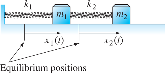
FIGURE 7.5.3.
The mass-and-spring system of Example 1.
The characteristic equation of A is
so A has the negative eigenvalues λ1=−25
Case 1: λ1=−25.
so an eigenvector associated with λ1=−25 is v1=[12]T.
Case 2: λ2=−100.
so an eigenvector associated with λ2=−100 is v2=[1−1]T.
By Eq. (11) it follows that a general solution of the system in (13) is given by
The two terms on the right in Eq. (14) represent free oscillations of the mass-and-spring system. They describe the physical system’s two natural modes of oscillation at its two [circular] natural frequencies ω1=5 and ω2=10.
(with c1=√a21+b21,cosα1=a1/c1,
and therefore describes a free oscillation in which the two masses move in synchrony in the same direction and with the same frequency ω1=5,
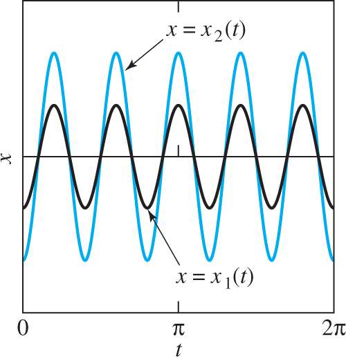
FIGURE 7.5.4.
Oscillations in the same direction with frequency ω1=5;
has the scalar component equations
and therefore describes a free oscillation in which the two masses move in synchrony in opposite directions with the same frequency ω2=10
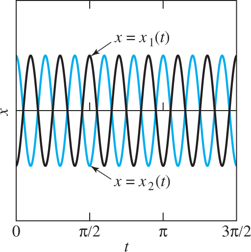
FIGURE 7.5.5.
Oscillations in opposite directions with frequency ω2=10;
Example 2
Railway cars Figure 7.5.6 shows three railway cars connected by buffer springs that react when compressed, but disengage instead of stretching. With n=3,k2=k3=k,
which is equivalent to
with
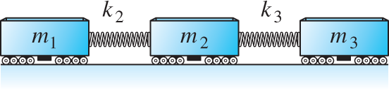
FIGURE 7.5.6.
The three railway cars of Example 2.
If we assume further that m1=m3,
for the characteristic equation of the coefficient matrix A in Eq. (18). Hence the matrix A has eigenvalues
corresponding to the natural frequencies
of the physical system.
For a numerical example, suppose that the first and third railway cars weigh 12 tons each, that the middle car weighs 8 tons, and that the spring constant is k=1:5
and
Hence the coefficient matrix A is
and the eigenvalue-frequency pairs given by (21a) and (21b) are λ1=0,ω1=0;λ2=−4,ω2=2;
Case 1: λ1=0,ω1=0.
so it is clear that v1=[111]T
Case 2: λ2=−4,ω2=2.
so it is clear that v2=[10−1]T
Case 3: λ3=−16,ω3=4.
so it is clear that v3=[1−31]T
The general solution x=x1+x2+x3 of x″=Ax
To determine a particular solution, let us suppose that the leftmost car is moving to the right with velocity v0
Then substitution of (24a) in (23) gives the scalar equations
which readily yield a1=a2=a3=0.
and their velocity functions are
Substitution of (24b) in (26) gives the equations
that readily yield b1=38v0, b2=14v0,
But these equations hold only so long as the two buffer springs remain compressed; that is, while both
To discover what this implies about t, we compute
and, similarly,
It follows that x2−x1<0 and x3−x2<0 until t=π/2≈1.57 (seconds), at which time the equations in (26) and (27) give the values
We conclude that the three railway cars remain engaged and moving to the right until disengagement occurs at time t=π/2. Thereafter, cars 1 and 2 remain at rest (!), while car 3 continues to the right with speed v0. If, for instance, v0=48 feet per second (about 33 miles per hour), then the three cars travel a distance of 9π≈28.27 (ft) during their 1:57 seconds of engagement, and
for t>π/2. Figure 7.5.7 illustrates the “before” and “after” situations, and Fig. 7.5.8 shows the graphs of the functions x1(t),x2(t), and x3(t) in Eqs. (27) and (27′).
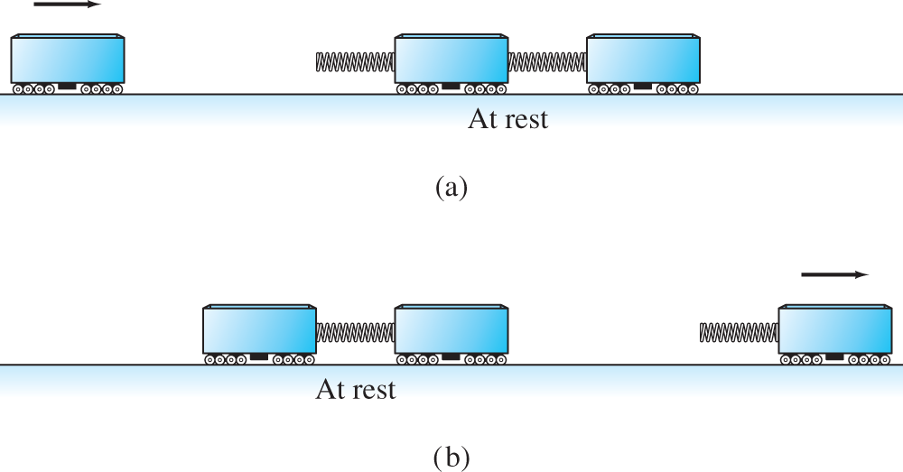
FIGURE 7.5.7.
(a) Before; (b) after.
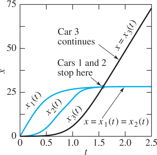
FIGURE 7.5.8.
Position functions of the three railway cars of Example 2.
Forced Oscillations and Resonance
Suppose now that the ith mass of the mass-and-spring system in Fig. 7.5.2 is subject to an external force Fi(i=1,2,…,n) in addition to the forces exerted by the springs attached to it. Then the homogeneous equation Mx″=Kx is replaced with the nonhomogeneous equation
where F=[F1F2…Fn]T is the external force vector for the system. Multiplication by M−1 yields
where f is the external force vector per unit mass. We are especially interested in the case of a periodic external force
(where F0 is a constant vector). We then anticipate a periodic particular solution
with the known external frequency ω and with a coefficient vector c yet to be determined. Because x″p=−ω2c cos ωt, substitution of (30) and (31) in (29), followed by cancellation of the common factor cos ωt, gives the linear system
to be solved for c.
Observe that the matrix A+ω2I is nonsingular—in which case Eq. (32) can be solved for c—unless −ω2=λ, an eigenvalue of A. Thus a periodic particular solution of the form in Eq. (31) exists provided that the external forcing frequency does not equal one of the natural frequencies ω1,ω2,…,ωn of the system. The case in which ω is a natural frequency corresponds to the phenomenon of resonance discussed in Section 5.6.
Example 3
Mass-spring resonance Suppose that the second mass in Example 1 is subjected to the external periodic force 50 cos ωt. Then with m1=2, m2=1, k1=100, k2=50, and F0=50 in Fig. 7.5.9, Eq. (29) takes the form

FIGURE 7.5.9.
The forced mass-and-spring system of Example 3.
and the substitution x=c cos ωt leads to the equation
for the coefficient vector c=[c1c2]T. This system is readily solved for
For instance, if the external squared frequency is ω2=50, then (35) yields c1=−1, c2=−1. The resulting forced periodic oscillation is described by
Thus the two masses oscillate in synchrony with equal amplitudes and in the same direction.
If the external squared frequency is ω2=125, then (35) yields c1=12, c2=−1. The resulting forced periodic oscillation is described by
and now the two masses oscillate in synchrony in opposite directions, but with the amplitude of motion of m2 twice that of m1.
It is evident from the denominators in (35) that c1 and c2 approach +∞ as ω approaches either of the two natural frequencies ω1=5 and ω2=10 (found in Example 1). Figure 7.5.10 shows a plot of the amplitude √c21+c22 of the forced periodic solution x(t)=c cos ωt as a function of the forced frequency ω. The peaks at ω2=5 and ω2=10 exhibit visually the phenomenon of resonance.

FIGURE 7.5.10.
Frequency–amplitude plot for Example 3.
Periodic and Transient Solutions
It follows from Theorem 4 of Section 7.2 that a particular solution of the forced system
will be of the form
![]()
where xp(t) is a particular solution of the nonhomogeneous system and xc(t) is a solution of the corresponding homogeneous system. It is typical for the effects of frictional resistance in mechanical systems to damp out the complementary function solution xc(t), so that
Hence xc(t) is a transient solution that depends only on the initial conditions; it dies out with time, leaving the steady periodic solution xp(t) resulting from the external driving force:
As a practical matter, every physical system includes frictional resistance (however small) that damps out transient solutions in this manner.
7.5 Problems
Problems 1 through 7 deal with the mass-and-spring system shown in Fig. 7.5.11 with stiffness matrix
and with the given mks values for the masses and spring constants. Find the two natural frequencies of the system and describe its two natural modes of oscillation.
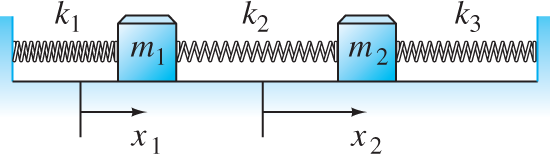
FIGURE 7.5.11.
The mass-and-spring system for Problems 1 through 6.
m1=m2=1; k1=0, k2=2, k3=0 (no walls)
m1=m2=1; k1=1, k2=4, k3=1
m1=1, m2=2; k1=1, k2=k3=2
m1=m2=1; k1=1, k2=2, k3=1
m1=m2=1; k1=2, k2=1, k3=2
m1=1, m2=2; k1=2, k2=k3=4
m1=m2=1; k1=4, k2=6, k3=4
In Problems 8 through 10 the indicated mass-and-spring system is set in motion from rest (x′1(0)=x′2(0)=0) in its equilibrium position (x1(0)=x2(0)=0) with the given external forces F1(t) and F2(t) acting on the masses m1 and m2, respectively. Find the resulting motion of the system and describe it as a superposition of oscillations at three different frequencies.
The mass-and-spring system of Problem 2, with F1(t)=96 cos 5t, F2(t)≡0
The mass-and-spring system of Problem 3, with F1(t)≡0, F2(t)=120 cos 3t
The mass-and-spring system of Problem 7, with F1(t)=30 cos t, F2(t)=60 cos t
Consider a mass-and-spring system containing two masses m1=1 and m2=1 whose displacement functions x(t) and y(t) satisfy the differential equations
x″=−40x+8y,y″=12x−60y.(a) Describe the two fundamental modes of free oscillation of the system. (b) Assume that the two masses start in motion with the initial conditions
x(0)=19,x′(0)=12and
y(0)=3,y′(0)=6and are acted on by the same force, F1(t)=F2(t)=−195 cos 7t. Describe the resulting motion as a superposition of oscillations at three different frequencies.
In Problems 12 and 13, find the natural frequencies of the three-mass system of Fig. 7.5.1, using the given masses and spring constants. For each natural frequency ω, give the ratio a1:a2:a3 of amplitudes for a corresponding natural mode x1=a1cos ωt, x2=a2cos ωt, x3=a3cos ωt.
m1=m2=m3=1; k1=k2=k3=k4=1
m1=m2=m3=1; k1=k2=k3=k4=2 (Hint: One eigenvalue is λ=−4.)
In the system of Fig. 7.5.12, assume that m1=1, k1=50, k2=10, and F0=5 in mks units, and that ω=10. Then find m2 so that in the resulting steady periodic oscillations, the mass m1 will remain at rest(!). Thus the effect of the second mass-and-spring pair will be to neutralize the effect of the force on the first mass. This is an example of a dynamic damper. It has an electrical analogy that some cable companies use to prevent your reception of certain cable channels.

FIGURE 7.5.12.
The mechanical system of Problem 14.
Suppose that m1=2, m2=12, k1=75, k2=25, F0=100, and ω=10 (all in mks units) in the forced mass-and-spring system of Fig. 7.5.9. Find the solution of the system Mx″=Kx+F that satisfies the initial conditions x(0)=x′(0)=0.
In Problems 16 through 19 we apply the analysis of Example 2 to a system of two railway cars.
Figure 7.5.13 shows two railway cars with a buffer spring. We want to investigate the transfer of momentum that occurs after car 1 with initial velocity v0 impacts car 2 at rest. The analog of Eq. (18) in the text is
x″=[−c1c1c2−c2] xwith ci=k/mi for i=1, 2. Show that the eigenvalues of the coefficient matrix A are λ1=0 and λ2=−c1−c2, with associated eigenvectors v1=[11]T and v2=[c1−c2]T.

FIGURE 7.5.13.
The two railway cars of Problems 16 through 19.
If the two cars of Problem 16 both weigh 16 tons (so that m1=m2=1000 (slugs)) and k=1 ton/ft (that is, 2000 lb/ft), show that the cars separate after π/2 seconds, and that x′1(t)=0 and x′2(t)=v0 thereafter. Thus the original momentum of car 1 is completely transferred to car 2.
If cars 1 and 2 weigh 8 and 16 tons, respectively, and k=3000 lb/ft, show that the two cars separate after π/3 seconds, and that
x′1(t)=−13v0andx′2(t)=+23v0thereafter. Thus the two cars rebound in opposite directions.
If cars 1 and 2 weigh 24 and 8 tons, respectively, and k=1500 lb/ft, show that the cars separate after π/2 seconds, and that
x′1(t)=+12v0andx′2(t)=+32v0thereafter. Thus both cars continue in the original direction of motion, but with different velocities.
Problems 20 through 23 deal with the same system of three railway cars (same masses) and two buffer springs (same spring constants) as shown in Fig. 7.5.6 and discussed in Example 2. The cars engage at time t=0 with x1(0)=x2(0)=x3(0)=0 and with the given initial velocities (where v0=48ft/s). Show that the railway cars remain engaged until t=π/2 (s), after which time they proceed in their respective ways with constant velocities. Determine the values of these constant final velocities x′1(t), x′2(t), and x′3(t) of the three cars for t>π/2. In each problem you should find (as in Example 2) that the first and third railway cars exchange behaviors in some appropriate sense.
x′1(0)=v0, x′2(0)=0, x′3(0)=−v0
x′1(0)=2v0, x′2(0)=0, x′3(0)=−v0
x′1(0)=v0, x′2(0)=v0, x′3(0)=−2v0
x′1(0)=3v0, x′2(0)=2v0, x′3(0)=2v0
In the three-railway-car system of Fig. 7.5.6, suppose that cars 1 and 3 each weigh 32 tons, that car 2 weighs 8 tons, and that each spring constant is 4 tons/ft. If x′1(0)=v0 and x′2(0)=x′3(0)=0, show that the two springs are compressed until t=π/2 and that
x′1(t)=−19v0andx′2(t)=x′3(t)=+89v0thereafter. Thus car 1 rebounds, but cars 2 and 3 continue with the same velocity.
The Two-Axle Automobile
In Example 4 of Section 5.6 we investigated the vertical oscillations of a one-axle car—actually a unicycle. Now we can analyze a more realistic model: a car with two axles and with separate front and rear suspension systems. Figure 7.5.14 represents the suspension system of such a car. We assume that the car body acts as would a solid bar of mass m and length L=L1+L2. It has moment of inertia I about its center of mass C, which is at distance L1 from the front of the car. The car has front and back suspension springs with Hooke’s constants k1 and k2, respectively. When the car is in motion, let x(t) denote the vertical displacement of the center of mass of the car from equilibrium; let θ(t) denote its angular displacement (in radians) from the horizontal. Then Newton’s laws of motion for linear and angular acceleration can be used to derive the equations
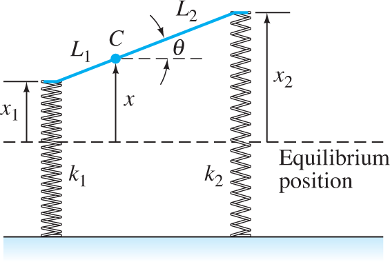
FIGURE 7.5.14.
Model of the two-axle automobile.
Suppose that m=75 slugs (the car weighs 2400 lb), L1=7 ft, L2=3 ft (it’s a rear-engine car), k1=k2=2000 lb/ft, and I=1000 ft·lb·s2. Then the equations in (40) take the form
75x″+4000x−8000θ=0,1000θ″−8000x+116,000θ=0.(a) Find the two natural frequencies ω1 and ω2 of the car. (b) Now suppose that the car is driven at a speed of v feet per second along a washboard surface shaped like a sine curve with a wavelength of 40 ft. The result is a periodic force on the car with frequency ω=2πv/40=πv/20. Resonance occurs when ω=ω1 or ω=ω2. Find the corresponding two critical speeds of the car (in feet per second and in miles per hour).
Suppose that k1=k2=k and L1=L2=12L in Fig. 7.5.14 (the symmetric situation). Then show that every free oscillation is a combination of a vertical oscillation with frequency
ω1=√2k/mand an angular oscillation with frequency
ω2=√kL2/(2I).
In Problems 27 through 29, the system of Fig. 7.5.14 is taken as a model for an undamped car with the given parameters in fps units. (a) Find the two natural frequencies of oscillation (in hertz). (b) Assume that this car is driven along a sinusoidal washboard surface with a wavelength of 40 ft. Find the two critical speeds.
m=100, I=800, L1=L2=5, k1=k2=2000
m=100, I=1000, L1=6, L2=4, k1=k2=2000
m=100, I=800, L1=L2=5, k1=1000, k2=2000
7.5 Application Earthquake-Induced Vibrations of Multistory Buildings
In this application you are to investigate the response to transverse earthquake ground oscillations of the seven-story building illustrated in Fig. 7.5.15. Suppose that each of the seven (above-ground) floors weighs 16 tons, so the mass of each is m=1000 (slugs). Also assume a horizontal restoring force of k=5 (tons per foot) between adjacent floors. That is, the internal forces in response to horizontal displacements of the individual floors are those shown in Fig. 7.5.16. It follows that the free transverse oscillations indicated in Fig. 7.5.15 satisfy the equation Mx″=Kx with n=7, mi=1000 (for each i), and ki=10,000 (lb/ft) for 1≦i≦7. The system then reduces to the form x″=Ax with

FIGURE 7.5.15.
The seven-story building.
Once the matrix A has been entered, the TI-Nspire command eigVl(A) instantly computes the seven eigenvalues shown in the λ-column of the table in Fig. 7.5.17. Alternatively, you can use the Maple command eigenvals(A), the Matlab command eig(A), or the Mathematica command Eigenvalues[A].
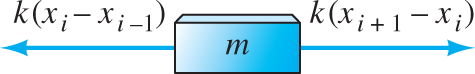
FIGURE 7.5.16.
Forces on the ith floor.
FIGURE 7.5.17.
Frequencies and periods of natural oscillations of the seven-story building.
| Eigenvalue | Frequency | Period | |
|---|---|---|---|
| i | λ | ω=√−λ | P=2πω(sec) |
| 1 | −38.2709 | 6.1863 | 1.0157 |
| 2 | −33.3826 | 5.7778 | 1.0875 |
| 3 | −26.1803 | 5.1167 | 1.2280 |
| 4 | −17.9094 | 4.2320 | 1.4847 |
| 5 | −10.0000 | 3.1623 | 1.9869 |
| 6 | −3.8197 | 1.9544 | 3.2149 |
| 7 | −0.4370 | 0.6611 | 9.5042 |
Then calculate the entries in the remaining columns of the table showing the natural frequencies and periods of oscillation of the seven-story building. Note that a typical earthquake producing ground oscillations with a period of 2 seconds is uncomfortably close to the fifth natural frequency (with period 1.9869 seconds) of the building.
A horizontal earthquake oscillation Ecos ωt of the ground, with amplitude E and acceleration a=−Eω2 cos ωt, produces an opposite inertial force F=ma=mEω2 cos ωt on each floor of the building. The resulting nonhomogeneous system is
where b=[1111111]T and A is the matrix of Eq. (1). Figure 7.5.18 shows a plot of maximal amplitude (for the forced oscillations of any single floor) versus the period of the earthquake vibrations. The spikes correspond to the first six of the seven resonant frequencies. We see, for instance, that whereas an earthquake with period 2 (s) likely would produce destructive resonance vibrations in the building, it probably would be unharmed by an earthquake with period 2.5 (s). Different buildings have different natural frequencies of vibration, and so a given earthquake may demolish one building but leave untouched the one next door. This seeming anomaly was observed in Mexico City after the devastating earthquake of September 19, 1985.
For your personal seven-story building to investigate, let the weight (in tons) of each story equal the largest digit of your student ID number and let k (in tons/ft) equal the smallest nonzero digit. Produce numerical and graphical results like those illustrated in Figs. 7.5.17 and 7.5.18. Is your building susceptible to likely damage from an earthquake with period in the 2- to 3-second range?

FIGURE 7.5.18.
Resonance vibrations of a seven-story building—maximal amplitude as a function of period.
You might like to begin by working manually the following warm-up problems.
Find the periods of the natural vibrations of a building with two above-ground floors, each weighing 16 tons and with each restoring force being k=5 tons/ft.
Find the periods of the natural vibrations of a building with three above-ground floors, with each weighing 16 tons and with each restoring force being k=5 tons/ft.
Find the natural frequencies and natural modes of vibration of a building with three above-ground floors as in Problem 2, except that the upper two floors weigh 8 tons each instead of 16. Give the ratios of the amplitudes A, B, and C of oscillations of the three floors in the form A:B:C with A=1.
Suppose that the building of Problem 3 is subject to an earthquake in which the ground undergoes horizontal sinusoidal oscillations with a period of 3 s and an amplitude of 3 in. Find the amplitudes of the resulting steady periodic oscillations of the three above-ground floors. Assume the fact that a motion Esin ωt of the ground, with acceleration a=−Eω2 sin ωt, produces an opposite inertial force F=−ma=mEω2 sin ωt on a floor of mass m.