7.2 Convex Geometry-Based Endmember Extraction

Due to the nature of a mixed sample vector in a linear mixing model, convex geometry has been used as a major criterion behind EEA design. As a simple illustrative example, assume that e₁ and e₂ are two endmembers. Any data sample vector x lying in a line segment connecting these two endmembers as end points can be expressed as a point linearly mixed by e₁ and e₂ and described in the form of , with based on convexity. For three endmembers e₁, e₂, and e₃, a data sample vector that is linearly mixed by these three endmembers must lie in a triangle with e₁, e₂, and e₃ as its three vertices. Similarly, a data sample vector within a triangular pyramid/tetrahedron, square-pyramid, and p-vertex simplex is also considered to be linearly mixed by its four vertices, five vertices, and p vertices, respectively, all of which are considered as endmembers. The OP and simplex volume are two principal criteria to materialize the concept of convex geometry.

7.2.1 Convex Geometry-Based Criterion: Orthogonal Projection

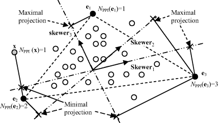
PPI is a popular technique widely used in endmember extraction due to its availability in the ENVI software provided by the Research Systems. Also due to its propriety and limited publication, its detailed implementation has never been made available in the public domain. Therefore, most people who use PPI for endmember extraction either appeal for the ENVI software or implement their own versions of PPI based on whatever available in the literature. Its idea is to use OP to determine whether a data sample vector is an endmember. If a data sample is a potential endmember, its OP on a random vector should be very likely to yield either maximal or minimal projection. In order to produce such a vector, a random unit vector is generated by PPI, referred to as a skewer. Figure 7.1 shows that the three skewers. skewer₁, skewer₂, and skewer₃, are randomly generated unit vectors where data sample vectors are denoted by open circles and three endmembers e₁, e₂, and e₃ by solid circles located at three vertices of the triangles and a maximal or a minimal projection of an endmember on a skewer is indicated by a cross “x.”

Figure 7.1 An illustration of PPI with three endmembers e₁, e₂, and e₃.

One of the major issues in PPI is sensitivity of two parameters used by PPI, which are K, the number of so-called skewers required for implementation, and τ, the cut-off threshold value for the scores, that is, counts produced by PPI, to extract candidate pixel vectors for final selection of endmembers. Another issue is the requirement of human intervention to manually select a final set of endmembers via a visualization tool provided by ENVI. Most importantly, PPI is a one-shot process, not an iterative process. Therefore, previous PPI-generated results cannot be used for next-stage new generation of endmembers if the number of skewers is increased.

This section presents our experience with PPI to offer our understanding of the ENVI's PPI and provide our version of its implementation so that those who are interested in PPI can easily implement them to repeat our experimental results without appealing for particular software. In the mean time, we also investigate several issues resulting from its implementation. Since the MATLAB is the major software in engineering, it is highly desirable to develop a MATLAB-based PPI algorithm as described below to implement in the same way as ENVI's PPI does.

One difference between the original PPI and the MATLAB-PPI is that the former provides no guideline to select the number of dimensions or components required to be retained after DR, while the latter uses VD to estimate the value of q for DR. In addition, the proposed MATLAB-based PPI algorithm also allows users to keep track of the PPI count for each of sample pixel vectors, which is defined as the number of skewers on which the pixel vector is orthogonally projected and falls at their ends, compared to the ENVI's PPI that does not automatically provide PPI counts for all the sample pixel vectors (i.e., we need to do it manually). Our MATLAB-based PPI is verified by PPI in the ENVI in the sense that both produced very close results.

MATLAB PPI Algorithm

1. Initialization:

i. Use VD to determine the number of dimensions, q, required to be retained after DR.

ii. Apply a DR technique such as a maximum noise fraction (MNF) transform (Green et al., 1988; Lee et al. 1990) to reduce the dimensionality of the data set to q component images.

iii. Randomly generate a set of K unit vectors, called “skewers,” where K is a preassumed sufficiently large positive integer.

2. PPI count calculation:

Project all the data sample vectors orthogonally onto all the skewers . Then for each data sample vector r, find those skewers on which the r produces either the maximal or minimal projection at their end points. These skewers form a set, called S_extrema(r), for the r. The PPI count of the r is defined as the number of skewers in S_extrema(r), that is,

(7.1)

where |A| is defined as the number of elements in a set A.

3. Candidate selection:

Find an appropriate value t to threshold the PPI count for all the sample vectors to select potential candidates for endmembers.

4. Endmember extraction:

Extract all the sample vectors with as endmembers.

In order to illustrate the steps implemented in the MATLAB PPI, let be a given set of data sample vectors. For a given value of K a random generator is used to produce a set of K random unit vectors, referred to as skewers, , which cover K different random directions. All the data sample vectors are then orthogonally projected on this randomly generated skewer set, . According to geometry of convexity, an endmember that is considered as a pure signature should occur at end points of some of these skewers with either maximal or minimal projection. For each sample vector r_i we further calculate the number of skewers, denoted by N_PPI(r_i), at which this particular sample vector occurs as an end point to tally the PPI count for r_i. As an example by letting K = 3, three skewers, skewer₁, skewer₂, and skewer₃, are randomly generated as shown in Figure 7.1. Assume that the data sample vectors are denoted by open circles. Then each of these data sample vectors is projected on these three skewers to see whether it yields maximal or minimal projection. For example, the data sample vector indicated by e₃ has two maximal projections along skewers skewer₁ and skewer₂, and one minimal projection on skewer skewer₃. So, in this case, its PPI count is N_PPI(e₃) = 3. Similarly, the data sample vector indicated by e₂ produces minimal projections on two skewers, skewer₁ and skewer₂, but neither maximal nor minimal projection on skewer₃. This gives e₂ a PPI count, N_PPI(e₂) = 2. In addition, the data sample vector indicated by e₁ produces maximal projection on skewer₃, but neither maximal nor minimal projection on the other two skewers, skewer₁ and skewer₂. As a result, its PPI count, N_PPI(e₁) = 1. Except these three data sample vectors e₁, e₂, and e₃ shown by solid circles none of data sample vectors shown by open circles can produce nonzero PPI counts. Interestingly, there is a data sample vector shown by a gray circle and specified by x that also produces N_PPI(e₁) = 1. However, if we calculate the volumes formed by various triangles with their vertices selected from three out of these four data sample vectors, e₁, e₂, e₃, and x, the only one triangle specified by dashed lines and formed by the three vertices, e₁, e₂, and e₃ produces the maximal volume. This indicates that e₁, e₂, and e₃ are the three desired endmembers.

Because of convexity, all the sample vectors in Figure 7.1 inside the triangle are supposed to have their PPI counts = 0, which implies that they are mixtures of the three endmembers at the vertices of the triangle indicated by dashed lines. It should be noted that a projection can be positive or negative depending on whether the projection occurs in the same or opposite direction of a skewer. A data sample with its maximal or minimal projection that occurred at a skewer is the one that is a potential candidate for an endmember.

Obviously, the above PPI algorithm is not an iterative process. It is performed for a given set of K skewers. Once it is done, the process is terminated. In order to ensure that our MATLAB PPI algorithm operates in the same way as the ENVI's PPI does, all the steps described above have been verified via experiments by PPI in the ENVI 3.6 version with no use of a visualization tool provided in ENVI's PPI, in which case both versions produce the same results. Finally, PPI extracts endmembers according to their PPI counts, which are thresholded by a value t that must be determined a priori. As a result, all sample vectors whose PPI counts are higher than t will be extracted as endmembers. In this case, many endmembers representing the same pure signature may also be extracted.

In what follows, we summarize several drawbacks resulting from the PPI in ENVI.

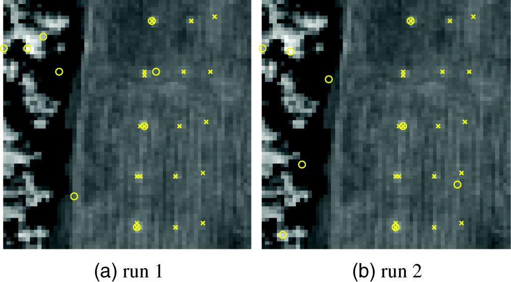
Figures 7.2 and 7.3 show two runs of HYDICE data in Figure 1.15(a) results by MATLAB-PPI using 200 and 1000 skewers, respectively, where four DR methods, PCA, MNF, SVD, and ICA, were used to perform DR.

Figure 7.2 Panel pixels extracted by MATLAB-PPI with 200 skewers with two different runs using PCA, MNF, SVD, and ICA.

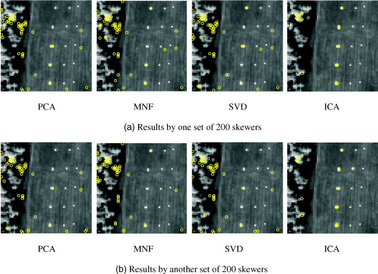
Figure 7.3 Panel pixels extracted by MATLAB-PPI with 1000 skewers with two different runs using PCA, MNF, SVD and ICA.

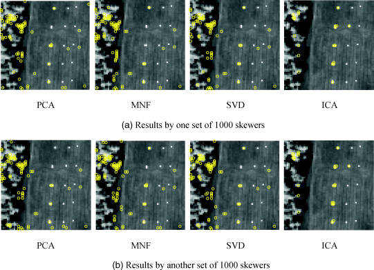
As shown in Figures 7.2 and 7.3, only PPI using ICA to perform DR could extract panel pixels, representing five endmembers in both cases of 200 and 1000 skewers. Three interesting findings observed from Figures 7.2 and 7.3 are worthwhile.

7.2.2 Convex Geometry-Based Criterion: Minimal Simplex Volume

In addition to the OP criterion described in Section 7.2.1, another way to realize the convex geometry is to use the simplex volume as a measure to determine whether a set of data sample vectors are desired endmembers. If there are p endmembers in the data space, two criteria can be used for simplex volume measure. One is to find a set of p endmembers whose simplex volume is minimal among all possible p-vertex simplexes that embrace all data sample vectors. In other words, it begins with an initial simplex that includes all data sample vectors and then gradually deflates simplexes by replacing data sample vectors repeatedly until it reaches a simplex with minimal volume while still embracing all data sample vectors, in which case the vertices of the resulting simplex are assumed to be endmembers. This is an early approach used in MVT (Crag, 1994) and CCA (Ifarragaerri and Chang, 1999), and will be briefly described below.

7.2.2.1 Minimal-Volume Transform (MVT)

The minimal-volume transform (MVT) proposed by Craig (1994) is a nonorthogonal linear transformation that transforms the image data to a new set of coordinates with the origin set to be at so-called dark point so that the new coordinate planes can embrace the data as tightly as possible. In doing so, two linear nonorthogonal transforms, called dark-point-fixed (DPF) transform and fixed-point-free (FPF) transform, are introduced to carry out the MVT transform. The DPF transform is based on absolute coordinates centered at the origin, while the FPF transform is barycentric center at the data. The connection of MVT with linear unmixing is to find endmembers so that data samples can be circumscribed by the minimal-volume data simplex formed by the set of endmembers.

7.2.2.2 Convex Cone Analysis (CCA)

Convex cone analysis (CCA) was developed by Ifarragaerri and Chang (1999) for endmember extraction. Their idea is very similar to MVT. It also models individual component spectral signatures as vertices of a convex cone with spectra strictly non-negative. The vectors formed by the spectra that are inside the cone region will be considered to be mixed spectra. The objective of CCA is to find the boundaries of this region as defined by its vertices with minimal possible volume. The corner spectra are then the desired endmembers. In other words, CCA finds a convex cone with smallest possible volume that will embrace all data sample vectors resulting from mixtures of its vertices. It imposes a non-negativity constraint and finds the boundaries of the region that contains all positive linear combinations of the first p eigenvectors of a sample spectral correlation matrix R formed by , where p is the number of endmembers to be generated, N is the total number of L-dimensional pixel vectors in the entire image data, L is the total number of spectral bands, and X is a normalized data matrix formed by . For a given set of p L-dimensional eigenvectors of the matrix R with , CCA solves a set of L algebraic equations

(7.2)

for p–1 abundance fractions with for . Since the exact solution for can be only found by exhausting p–1 equations among the L algebraic equations, there are combinations of equations that need to be solved for . These solutions will produce linear combinations of the eigenvectors that have at least p–1 zeros. So, a boundary occurs when at least one of the vector elements in the linear combination of eigenvectors is zero while the other elements are non-negative. It should be noted that MVT and CCA share the same concept in the sense that the coordinate planes used in MVT to embrace data cloud correspond to the faces of the convex cone used in CCA. However, both MVT and CCA are different in essence. MVT finds endmembers that form a minimal-volume data simplex that circumscribes a mixing simplex formed by the same set of endmembers via linear unmixing, whereas CCA looks for corners or vertices of a convex cone that are as far away from each other as possible.

7.2.3 Convex Geometry-Based Criterion: Maximal Simplex Volume

As an alternative, a second simplex volume-based criterion is to find a simplex formed by a p- endmember simplex embedded in a data space whose volume is maximal among all possible p-vertex simplexes formed by any set of p data sample vectors. This approach can be considered as a simplex inflation process as opposed to the simplex deflation process used by MVT. It starts off with an initial simplex embedded in the data space and then keeps inflating simplexes within the data space by replacing vertices with other data sample vectors until it reaches a simplex whose volume is maximal, in which case the vertices of the found simplex are considered as endmembers. The best representative using this criterion is Winter's N-FINDR (Winter, 1999a,b). Since N-FINDR is preferred to other simplex-volume criteria in the literature, it will be described in detail in Section 7.2.4 along with its several variants.

The MVT and CCA described in Sections 7.2.2.1 and 7.2.2.2 make use of the nature in linear spectral unmixing (LSU) to find a minimal-volume data simplex to embrace all data sample vectors or data cloud via linear mixing. This section presents an idea slightly different from that used in MVT and CCA. Rather than finding a minimal-volume simplex to embrace data cloud from outside, it finds a maximal-volume simplex inside (i.e., embedded in) the data cloud so that the desired simplex can include as many data sample vectors as possible. The vertices of such found maximal-volume data simplex are designated as endmembers. In other words, a simplex with its all vertices specified by endmembers has the maximal volume compared to all simplexes embedded in the data space with same number of vertices. This is the key idea behind the N-FINDR developed by Winter (1999a,b). More specifically, within the data cloud N-FINDR finds a simplex whose volume is maximal among all simplexes with the same number of vertices. In this case, the vertices of a simplex with maximal volume are assumed to be endmembers. Unfortunately, a detailed step-by-step algorithmic implementation of N-FINDR was not provided in Winter (1999a,b). This is similar to the case of PPI where its detailed implementation is also missing. Following the same logical approach, we also develop several versions that can implement the Winter's N-FINDR, which will be referred to as simultaneous N-FINDR (SM N-FINDR).

7.2.3.1 Simultaneous N-FINDR (SM N-FINDR)

In this section, we summarize the steps to implement Winter's N-FINDR based on our understanding and experience. It by no means claims that our interpreted N-FINDR is identical to the one developed by Winter (1999a,b). Nevertheless, the idea used in both algorithms should be the same.

SM N-FINDR

1. Preprocessing.

a. Let p be the number of endmembers to be generated.

b. Apply a DR transform such as MNF to reduce the data dimensionality from L to p–1, where L is the total number of spectral bands.

2. Exhaustive search.

For any p data sample vectors form a p-vertex simplex specified by and define its volume, by

(7.3)

Find a set of p data sample vectors, denoted by , that yields the maximal value of (7.3), that is,

(7.4)

3. Let be the desired set of endmembers.

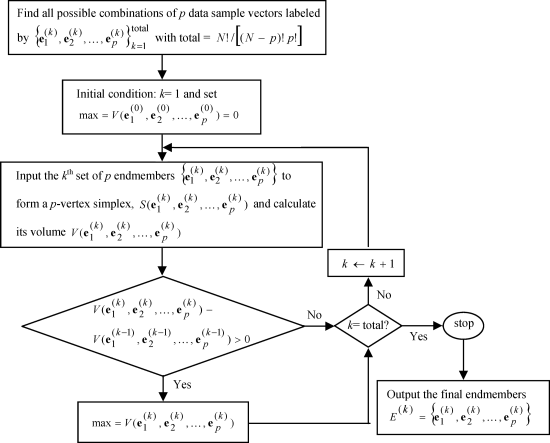
Figure 7.4 depicts a flow chart of implementing the SM N-FINDR.

Figure 7.4 A flow chart of SM N-FINDR implementation.

7.2.3.2 Iterative N-FINDR (IN-FINDR)

According to step 2 described in the above SM N-FINDR an exhaustive search must be conducted via (7.4) by finding an optimal set of endmembers, that requires tremendous computing time to accomplish this process. One way to mitigate this dilemma is to break up the exhaustive search process into two processes, inner loop and outer loop, each of which can be implemented iteratively. The resulting N-FINDR is called iterative N-FINDR (IN-FINDR) and can be described as follows.

Iterative N-FINDR (IN-FINDR)

1. Preprocessing.

a. Let p be the number of endmembers to be generated.

b. Apply a DR transform such as MNF to reduce the data dimensionality from L to p–1, where L is the total number of spectral bands.

2. Initialization.

Let be a set of initial vectors randomly selected from the data. .

3. Outer Loop.

At iteration , find the volume of the simplex specified by the p vertices , defined by (7.3).

4. Inner loop.

For , we recalculate for all data sample vectors r. If none of these p recalculated volumes, , ,, , is greater than , no endmember in will be replaced. The algorithm is terminated. Otherwise, continue.

5. Replacement rule.

The endmember that is absent in the largest volume among the p simplexes, , ,..., , will be replaced by the sample vector r. Assume that such an endmember is denoted by . A new set of endmembers is then produced by letting and for . Let and go to step 3.

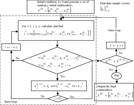
Figure 7.5 describes a flow chart of implementing IN-FINDR step by step in two loops, inner and outer loops.

Figure 7.5 A flow chart of IN-FINDR implementation.

Interestingly, a recent version of N-FINDR developed in Winter (2004) is actually implemented in two loops in a reverse order of the two loops carried out by the IN-FINDR.

It should be noted that the IN-FINDR developed in this section is generally not as optimal as SM N-FINDR. However, it can be considered as nearly optimal. The similarity between SM N-FINDR and IN-FINDR can be illustrated by the similarity between finding double integral and iterated integrals where the region to be integrated is generally a 2D dimensional space compared to the regions to be calculated by iterated integrals, which are usually one-dimensional space. Using this context as interpretation, the exhaustive search implemented in SM N-FINDR is similar to finding a multiple integral that integrates a multidimensional region in the original data space, whereas the inner and outer loops carried out in IN-FINDR iteratively are similar to finding iterated integrals over one-dimensional space. In most cases, the results obtained by iterated integrals are the same as those obtained by directly finding multiple integrals according to Fubini's theorem (Reed and Simon, 1972).

7.2.3.3 Various Versions of Implementing IN-FINDR

The replacement rule described in steps 4 and 5 of IN-FINDR is a general concept. For practical implementation the replacement rule can be designed to ease computation depending on how endmembers are replaced. There are several versions that can be designed to implement the replacement rule used by IN-FINDR. In this section, three variants of IN-FINDR are developed: single-replacement N-FINDR (1-IN-FINDR), multiple-replacement IN-FINDR, and successive IN-FINDR (SC IN-FINDR).

Single-Replacement IN-FINDR

The IN-FINDR presented in this section uses a simple replacement rule that replaces one endmember at a time. The resulting IN-FINDR is referred to as 1-IN-FINDR and the IN-FINDR described in Section 7.2.4.2 can be further specified as follows.

Single-Replacement IN-FINDR (1-IN-FINDR)

1. Preprocessing.

a. Let p be the number of endmembers to be generated.

b. Apply a DR transformation to reduce the data dimensionality from L to p–1, where L is the total number of spectral bands.

2. Initialization.

Let be a set of initial vectors randomly generated from the data. Let

3. Form a simplex with as the p vertices and define as its volume defined by (7.3).

4. For find that yields the maximal volume of over all sample vectors r, that is,

(7.5)

while fixing other endmembers with .

5. Check whether

(7.6)

If yes, the algorithm is terminated. Otherwise, let . Set and go to step 3.

Multiple-Replacement IN-FINDR

In the 1-IN-FINDR described above, the replacement carried out in step 5 is done by one single endmember at a time for each iteration, which is the endmember found in step 4. It is a suboptimal algorithm to perform endmember replacement in step 5 to save computational complexity. A possible extension of 1-IN-FINDR is to replace two endmembers at a time rather than single replacement implemented in 1-IN-FINDR. The following algorithm is designed for this purpose. It is a two-replacement IN-FINDR (2-IN-FINDR) where the single endmember replacement process carried out in steps 4 and 5 in 1-IN-FINDR is replaced by two endmembers at a time for each iteration described in the following steps 4 and 5.

Two-Replacement IN-FINDR (2-IN-FINDR)

4. For each pair (i,j) with , find a pair of that yields the maximum volume of over all sample vectors r, that is,

(7.7)

while fixing other endmembers with . It generally requires an extensive search for an optimal pair to satisfy (7.7), which is very time-consuming. One way to alleviate such a searching process is to solve two endmembers successively as follows:

(7.8)

where the obtained by (7.8) may not be the same pair of obtained from (7.5), but their volumes are generally very close.

(7.6)

If yes, the algorithm is terminated. Otherwise, let and . Then set and go to step 3.

Once a 2-IN-FINDR is developed, it can be easily extended to multiple-replacement IN-FINDR where more than two endmembers can be replaced in steps 4 and 5 in 2-IN-FINDR. More specifically, for any given integer s with the multiple-replacement IN-FINDR can replace s endmembers simultaneously to generate its new endmembers for next iteration, referred to as s-IN-FINDR described below.

s-Replacement IN-FINDR (s-IN-FINDR)

4. For any given set of s components with find a set of s components of that yields the maximal volume of over all s vector sample vectors , that is,

(7.9)

while fixing other endmembers with . It generally requires an extensive search for an optimal pair to satisfy (7.6), which is very time-consuming. One way to alleviate such a searching process is to solve two endmembers successively as follows:

(7.10)

where obtained by (7.10) may not be the same set of obtained from (7.7), but their volumes are generally very close.

(7.6)

If yes, the algorithm is terminated. Otherwise, let

(7.11)

Then set and go to step 3.

It should be noted that as s is increased, the computational complexity of s-IN-FINDR also grows exponentially until it reaches p, that is, when the s-IN-FINDR becomes the original version of IN-FINDR that replaces p endmembers simultaneously specified by (7.10).

Successive IN-FINDR (SC IN-FINDR)

As noted in the s-IN-FINDR, a major issue in its implementation is computational cost, which is expected to be very high. In order to mitigate this problem, an alternative suboptimal version of s-IN-FINDR can be derived as follows by replacing the simultaneous replacement of s endmembers in step 5 implemented in the s-IN-FINDR with a successive s-endmember replacement that is analogous to (7.10) but more efficient at the expense of optimality.

s-Successive replacement N-FINDR (s-SC IN-FINDR)

1. Preprocessing.

a. Let p be the number of endmembers to be generated.

b. Apply a DR transformation to reduce the data dimensionality from L to p−1, where L is the total number of spectral bands.

2. Initialization.

Let be a set of initial vectors randomly generated from the data. Set

3. Form a simplex with as its p vertices with its volume defined by (7.3).

4. For any given set of s components with find that yields the maximal volume of over all sample vectors , while fixing other endmembers with and with . That is,

(7.12)

5. Check whether the stopping rule specified by (7.6) is satisfied. If yes, the algorithm is terminated. Otherwise, let

(7.13)

Set and go to step 3.

In particular, if , steps 4 and 5 in the above s-SC IN-FINDR can be further modified as follows

p-Successive replacement N-FINDR (p-SC IN-FINDR)

4. For find that yields the maximum volume of over all sample vectors r, while fixing other endmembers with and with .

That is,

(7.14)

5. Check whether the stopping rule specified by (7.6) is satisfied. If yes, the algorithm is terminated. Otherwise, use (7.13) and set . Then go to step 3.

The major difference between s-IN-FINDR and s-SC IN-FINDR is the equation used to generate a new endmember that yields the maximal simplex volume, (7.8) in s-IN-FINDR and (7.12) in s-SC IN-FINDR. More specifically, in (7.8) the endmembers other than are fixed at the original endmembers for . However, in (7.12), only the endmembers in (7.7) after are fixed at for or , while those endmembers with are updated and replaced by setting for . As a result, with an EEA, which implements step 4 without step 5 in the version of p-SC IN-FINDR, can be considered as a SQ-EEA which will be discussed in Chapter 8 in detail. Nevertheless, since both versions implement step 5 to avoid a possible trap in local optima, they both eventually produce close results except that p-SC IN-FINDR may converge faster than p-IN-FINDR.

7.2.3.4 Discussions on Various Implementation Versions of IN-FINDR

The main reason for developing various approaches to implementing IN-FINDR is the following. Since SM N-FINDR must conduct an exhaustive search among all data sample vectors to ensure that an optimal set of endmembers is produced at the end, even for a moderate size of hyperspectral data, this approach is nearly impossible to accomplish within limited computing resources. This is an inevitable issue encountered in most of SM-EEAs, specifically convex hull-based EEAs such as MVT and CCA. As an example, for N-FINDR to be an optimal EEA, it must find all p endmembers simultaneously among all possible combinations, of p endmembers with N being the total number of data sample vectors. As N grows very large, its computational complexity becomes increasingly formidable in reality. One way to resolve this dilemma is to limit its search process to a feasible region in which the desired endmembers are most likely to occur. In doing so, two loops are designed to replace the exhaustive search required by N-FINDR, which results in IN-FINDR. This can be seen in the two loops designed for s-IN-FINDR and s-SC IN-FINDR, both of which use inner loop indexed by j_l in step 4 and outer loop indexed by k in step 5 to accomplish what the SM N-FINDR does. The inner loop runs by replacing the (j_l)th endmember with the most probable endmember that yields the maximal volume of in s-IN-FINDR via (7.10) or in s-SC IN-FINDR via (7.12). When l = s, s-IN-FINDR and s-SC IN-FINDR check whether the stopping rule described by (7.6) is satisfied. If it is, then s-IN-FINDR and s-SC IN-FINDR are terminated. Otherwise, they go to the outer loop indexed by k by implementing a replacement rule described by (7.6) for s-IN-FINDR or (7.13) for s-SC IN-FINDR and setting to go back to the inner loop again in step 4. According to our extensive experimental studies it seems that the p-SC IN-FINDR is the best in the sense that the outer loop is designed to accomplish the same task as IN-FINDR does by repeatedly replacing a set of p endmembers found by the inner loop in a successive manner until it obtains the maximal simplex volume.

Interestingly, as discussed in Chapter 8, when only the inner loop of s-SC IN-FINDR is implemented without iterating the outer loop, s-SC IN-FINDR becomes a successive EEA, specifically s = p, s-SC IN-FINDR is reduced to SC IN-FINDR discussed in Section 7.2.3.3, while with s = 1 s-SC IN-FINDR is reduced to SC N-FINDR in Section 8.2.

7.2.3.5 Comparative Study Among Various Versions of IN-FINDR

In order to see how each of various versions of IN-FINDR works in terms of its performance and computation, it is worthwhile conducting experiments using the same computing environment. The data to be used for illustration is the HYDICE image in Figure 1.15. Since IN-FINDR requires a DR, four DR techniques, singular value decomposition (SVD), principal components analysis (PCA), MNF, and independent component analysis (ICA) discussed in Chapter 6, are used for experiments. Additionally, according to the results in Chapter 5, the effective dimensionality to be retained after DR is estimated by VD to be 9. Therefore, q = 9 is used for our experiments. Finally, due to the use of random initial endmembers by IN-FINDR the experiments are also conducted using two different sets of random initial conditions to demonstrate inconsistency in final selected endmembers as shown in Figures 7.6–7.8, which present the nine endmember extraction results of two runs from two different sets of random initial endmembers along with their computing times in parentheses.

As demonstrated in Figures 7.6–7.8, 9-SC IN-FINDR required the least time of 11.4 s on average as expected, while 1-IN-FINDR had the worst time of about 42.5 s on average, which was roughly four times in computation compared to that needed by 9-SC IN-FINDR. It is also demonstrated that all the three versions of IN-FINDR using ICA to perform DR could extract all the five endmembers regardless of what random initial endmembers were used for initialization. In addition, inconsistent results were clearly shown by two different runs. It is particularly evidential for the three versions of IN-FINDR with SVD used to reduce dimensionality where two endmembers were extracted in one run while three endmembers were extracted in another run.

7.2.3.6 Alternative SM N-FINDR

Also interestingly, SM N-FINDR can be modified by introducing a scale parameter δ that controls effectiveness of the abundance sum-to-one constraint (ASC) imposed on selected endmembers. The resulting SM N-FINDR is called alternative SM N-FINDR (ASM N-FINDR) and its idea is summarized in the following algorithmic implementation.

ASM N-FINDR Algorithm

1. Set p to the number of endmembers to be generated; L is the number of bands.

Let be set of initial endmembers.

2. Let be the set of p endmembers generated at iteration and be an kth p-endmember matrix. We define an matrix by augmenting the matrix using , which is a p-dimensional unity vector as follows:

(7.15)

where δ is a scalar parameter that is used to control effectiveness of the ASC. Generally, δ can be chosen to be , where for and N is the total number of image pixels in the image. Now we can form a matrix by

(7.16)

where and from (7.3).

The criterion used by ASM N-FINDR is to iterate the p endmembers and make the determinant, , as large as possible where the iterative process can be carried out in the same manner as described in steps 3–5 in SM N-FINDR with (7.4) being replaced by (7.16).

7.2.4 Convex Geometry-Based Criterion: Linear Spectral Mixture Analysis

Linear spectral mixture analysis (LSMA) has been widely used in remote sensing image classification where the least-squares error (LSE) is considered as an optimal criterion for LSMA. It is highly desirable if it can be also used as a criterion for endmember extraction. Two LSMA-based techniques are of interest and take completely opposite approaches. Assume that there are p endmembers present in the data. One was proposed by Berman et al. (2004), referred to as iterated constrained endmember (ICE) to minimize the unmixed error resulting from a p-vertex simplex while constraining the size of a simplex via the sum of Euclidean distance among all p selected endmembers instead of the simplex volume used by MVT and N-FINDR. The other approach developed in this section is based on an underlying assumption that the unmixed error using all p endmembers via LSMA is always greater than that caused by using any set of p signatures for LSMA regardless of whether or not these signatures are pure or mixed. Such resulting unmixed LSE is referred to as maximal linear spectral unmixed error (MLSUE). Furthermore, two abundance constraints, sum-to-one and non-negativity, must be also imposed on LSMA to satisfy the constraint of convexity. This leads to a natural choice proposed in Ji (2005), referred to as FCLS-EEA, which is derived from the fully constrained least-squares (FCLS) developed in Heinz and Chang (2001). FCLS-EEA is also known as unsupervised fully constrained least squares (UFCLS) in Chang (2003a). It first starts with p randomly select endmembers and then calculates error vectors from the difference between the endmembers and the linear mixture model mixed by other endmembers with abundance estimated by the FCLS. The error vectors are used as projection vectors to find a new endmember that has the maximal length on the projections. The details of the algorithm are described as follows.

FCLS-EEA Algorithm

1. Initialization.

Let p be the number of endmembers to generate and be a set of randomly generated initial endmembers.

2. At iteration , for each we assume that is a mixed pixel and can be represented by that is generated by the remaining p−1 endmembers, using the FCLS, that is, where the p−1 abundance fractions are obtained by the FCLS.

3. Subtract from to form an error vector , which will be used as a projection vector.

4. Project all image pixels onto the projection vector and find the pixel, that yields the maximum length, that is, . Let . We form a new set of p endmembers by letting for and

5. If . Otherwise, let . Go to step 2.

Figure 7.9 shows the results of nine endmembers extracted by FCLS-EEA using two different sets of random initial endmembers where inconsistency caused by random initial conditions in final selected endmembers was also evidential with two panel pixels extracted in the first run and only one panel pixel extracted in the second run.

Figure 7.6 1-IN-FINDR.

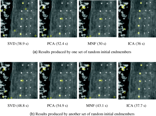
Figure 7.7 2-IN-FINDR.

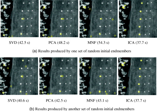
Figure 7.8 9-SC IN-FINDR.

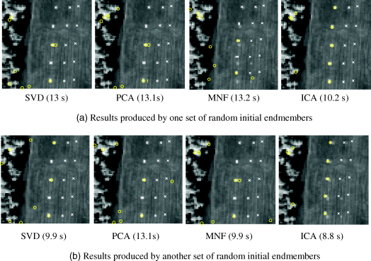
Figure 7.9 Nine endmembers extracted by the FCLS-EEA on the HYDICE data with two different runs.

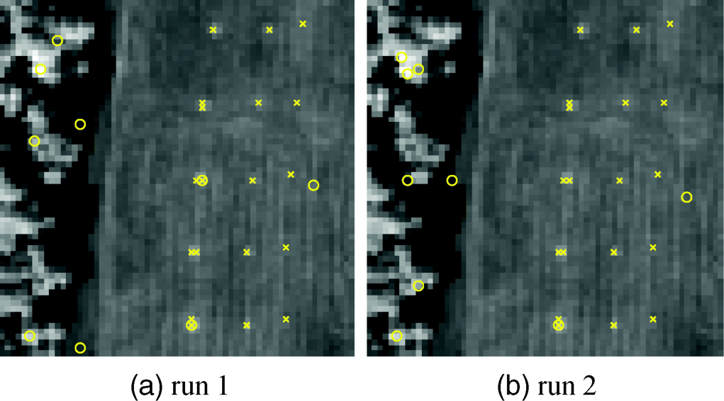
From Figure 7.9, it can be seen that FCLS-EEA did not work as well as it was designed for. Three major factors contribute to such poor performance.

In order to alleviate the second and third problems, OSP is applied as a new learning rule and the difference between error vectors in length is used as a stopping rule. Here, OSP is chosen to find a new endmember because it can find the most distinct candidate from the existing ones. Unlike the error vectors, the new endmember generated by OSP will not be the same at different iterations. In this case, the stopping rule takes advantage of an underlying principle for LSMA, that is, the error between a new real endmember found at (k + 1)st iteration and any data sample vector linearly unmixed by using previously found endmembers at the kth iteration is maximal. If the new endmember found at (k + 1)st iteration does not satisfy the condition, then the stopping rule terminates the algorithm. The above FCLS-EEA can be modified as follows.

FCLS-EEA Algorithm

1. Initialization.

Set p to be the number of endmembers to be generated.Let be a set of initial endmembers and be its corresponding endmember matrix.

2. At iteration k ≥ 0, apply an orthogonal subspace projector to all data sample vectors r and find a sample vector that yields the maximum orthogonal projection by

(7.17)

3. For 1 ≤ j ≤ p, assume that the jth endmember at the kth iteration, is not a pure signature but rather a mixed sample expressed as a linear mixture of all other endmembers, p−1 endmembers, given by

(7.18)

where are abundance fractions obtained by FCLS.

4. Calculate the error between the pure signature and the mixed signature by and find the index that yields the smallest error, that is, .

5. Now calculate the error vector and check whether ,

6. If it is, the algorithm is terminated and is the set of the final endmembers. Otherwise, let for and ; go to step 2.

Figure 7.10 shows the results of the modified FCLS-EEA with two different runs. The improvement is very obvious from these results.

Figure 7.10 Nine endmembers extracted by the modified FCLS-EEA on the HYDICE data with two different runs.