12.3 Gaussian Noise in OSP

The noise assumed in (12.1) is nothing more than additive, zero-mean, and white. More precisely, the noise assumed in (12.1) is uncorrelated with target signatures in M and is a zero-mean de-correlated (i.e., the noise covariance matrix is an identity matrix) random process. These two assumptions are not crucial and can be relaxed by data preprocessing. The assumption of additivity can be achieved by an estimation technique such as LS methods (Tu et al., 1997; Chang et al., 1998; Chang, 2003a) to remove correlation between target signal subspace and noise subspace. The assumption of zero-mean white noise can be accomplished by a prewhitening process described in Section 6.3.1, a widely used technique in communications and signal processing community (Poor, 1994). Since SNR is generally very high in hyperspectral imagery, the correlation of the noise subspace with the target signature subspace is significantly reduced compared to that in multispectral imagery. This may be one of the major reasons that OSP has been successful even though it violates the additivity assumption and white noise, but the consequence does not cause much performance deterioration. Nevertheless, by taking advantage of the Gaussian assumption many research efforts have produced satisfactory results (Tu et al., 1997; Chang et al., 1998; Chang, 2003a; Manolakis, 2001) as follows.

12.3.1 Signal Detector in Gaussian Noise Using OSP-Model

In this section, we investigate the role of Gaussian noise assumption in OSP. Specifically, when OSP-model is cast as a two-hypothesis (signal and noise) problem, OSP becomes a maximum likelihood detector. Moreover, if OSP is used as a signal estimator, it can further be shown to be equivalent to the maximum likelihood estimator, which includes the two-class Gaussian discriminant function as a special case.

In what follows, we assume that the noise in (12.1) is zero-mean Gaussian with the covariance matrix given by Σ_n. In this case, the probability distribution of r in (12.1) is a Gaussian distribution p(r|Mα) = N(Mα,Σ_n) with mean vector and covariance matrix given by Mα and Σ_n, respectively. Similarly, we can obtain the probability distribution for in OSP-model specified by (12.4), which is with . Using the OSP-model as a signal detection model, a standard signal detection problem can be formed by the following binary hypothesis test:

(12.31)

where and . Following a standard derivation in Poor (1994) a likelihood ratio test (LRT) Λ(z) resulting from (12.31) can be obtained by

(12.32)

However, any color Gaussian noise can further be simplified by the whitening process (Poor, 1994, pp. 58–60) or in Section 6.3.1 and reduced to a white Gaussian noise (WGN) with . In this case, the LRT Λ(z) in (12.32) becomes that has the same filter structure as δ^OSPD(r) specified by (12.9) and δ^OSP(r) specified by (12.17). Let the false alarm probability be denoted by P_F and define , then

(12.33)

that produces the threshold

(12.34)

The detection probability

(12.35)

turns out to be identical to the one derived in Tu et al. (1997), Chang et al. (1998), and Chang (2003a).

12.3.2 Gaussian Maximum Likelihood Classifier Using OSP-Model

Once again, OSP-model is used with . Let C₀ and C₁ represent two classes corresponding to noise and signal, respectively. Their discriminant functions can be specified by their corresponding a posteriori probability distributions given by for . In other words, z is assigned to class C₁, that is, if , and , otherwise. In this case, we can derive

(12.36)

where and , and and are prior probabilities of C₀ and C₁, respectively. Equation (36) turns out to be the LRT Λ(z) in (12.31) with the threshold given by . If we further assume that the prior probabilities and are equally likely, the discriminant function described by (12.36) is reduced to the maximum likelihood detector given by

(12.37)

With the Gaussian noise assumption (12.37) can be calculated and expressed as follows:

(12.38)

(12.39)

(12.40)

Equation (12.40) makes sense since we assume that the noise is zero-mean and the prior probabilities of the noise class C₀ and the signal class C₁ are equally likely. If we substitute for z in (12.40), then (12.40) becomes

(12.41)

where the left-hand side of (12.41) is exactly given by (12.22). In this case, Equation (12.41) can be considered as Gaussian discriminant function for (d,U)-model.

12.3.3 Gaussian Maximum Likelihood Estimator

Using the Gaussian noise assumed in OSP-model, the maximum likelihood estimate of the abundance fraction α_p, is then given by

(12.42)

where , , and as defined in (12.31). Solving (12.42) is equivalent to minimizing the following the Mahalanobis distance (Fukunaga, 1990):

(12.43)

that yields the solution

(12.44)

Substituting and using we obtain

(12.45)

Now, if the Gaussian noise is whitened, that is, , (12.45) becomes

(12.46)

that is exactly the same one derived in Settle (1996), Chang et al. (1998), and Chang (2003a). The abundance fraction of the desired target signature d is estimated by that can be obtained directly from the Gaussian maximum likelihood estimator and is identical to (12.24). The preprocessing of using to annihilate the undesired target signatures is not necessary for δ^GML(r) since it has been already taken care of in the LS estimator shown in (12.25). Once again, (12.46) includes a constant that accounts for the LS estimation error and is absent in δ^OSP(r) given by (12.17).

12.3.4 Examples

In what follows, we conduct experiments to examine the noise assumption used in OSP. Two scenarios will be simulated: white Gaussian noise versus white uniform noise (WUN) and color Gaussian noise versus white Gaussian noise.

Example 12.1

(White Gaussian Noise vs. White Uniform Noise)

This example demonstrates that the Gaussian noise is an unnecessary assumption for OSP. The set of five reflectance spectra shown in Figure 1.8 is used for illustration and contains five reflectance spectra: dry grass, red soil, creosote leaves, blackbrush, and sagebrush. A signature matrix M is formed by the dry grass, red soil, and creosote leaves signatures, with their associated abundance fractions denoted by . The simulation consisted of 401 mixed pixel vectors. We started the first pixel vector with 100% red soil and 0% dry grass, then began to increase 0.25% dry grass and decrease 0.25% red soil every pixel vector until the 401st pixel vector that contained 100% dry grass. We then added creosote leaves to pixel vector numbers 198–202 at abundance fractions 10% while reducing the abundance of red soil and dry grass by multiplying their abundance fractions by 90%. For example, after addition of creosote leaves, the resulting pixel vector 200 contained 10% creosote leaves, 45% red soil, and 45% dry grass. Two types of noise were simulated, white zero-mean Gaussian noise with variance σ²and white zero-mean uniform noise with its probability density function defined on [−a, a] and variance . They were added to each band to achieve the signal-to-noise ratio (SNR) defined in Harsanyi and Chang (1994) as 50% reflectance divided by the standard deviation of the noise. Figures 12.2 and 12.3 show the results of OSP detector, δ^OSP(r) and OSP estimator in these two types of noise, Gaussian noise and uniform noise with SNR = 30:1, 20:1, and 10:1.

As we can see from these figures, there was no visible difference between Gaussian noise and uniform noise. Table 12.1 also tabulates their corresponding results of δ^OSP(r) and in detecting creosote leaves where there was little difference in terms of LSE in abundance fractions between WGN and WUN produced by δ^OSP(r) and .

Nevertheless, the abundance fractions detected by δ^OSP(r) and estimated by were quite different where produced much more accurate estimates of abundance fractions than does δ^OSP(r). This was because the scale constant in was included to effectively account for estimation error.

Example 12.2

(Gaussian–Markov Noise)

According to the model specified by (12.1) the noise is assumed to be zero-mean and white. More specifically, the noise assumed in the (d,U)-model is additive and zero-mean. Its covariance matrix is also an identity matrix that implies that the band-to-band noise within a hyperspectral image pixel vector is uncorrelated. Interestingly, to the author's best knowledge, most of OSP-based techniques do not include a whitening process, but still successfully achieve their goals. These also include Harsanyi and Chang's OSP (Harsanyi and Chang, 1994). The reason is that due to high spectral resolution the signal-to-noise ratio is generally very high in hyperspectral imagery. In this case, the noise has little impact on OSP performance. Whether or not the noise is white becomes immaterial. This evidence is shown in the following experiments where the whitening process does improve the performance, but the gain is very small.

According to the OSP-model, the whitening was only performed on interband spectral correlation at the pixel level. In this case, a first-order zero-mean Gaussian–Markov noise (GMN) with the between-band correlation coefficient (CC) specified by ρ was added to each pixel vector simulated in Example 12.1 to achieve various levels of SNRs. The covariance matrix of such Gaussian–Markov noise has the form given by , that is:

(12.47)

Figures 12.4 and 12.5 show the results of δ^OSP(r) and operating in first-order Gaussian–Markov noise with different correlation coefficients specified by ρ in (12.47) and SNRs.

Table 12.2 also tabulates the detection results of creosote leaves by δ^OSP(r) and along with their respective LSEs. In addition, compared to Figures 12.2 and 12.3 and Table 12.1, δ^OSP(r) and performed slightly better in white nose than they did in color noise, but the improvements were very limited. The results also demonstrated that the performance of δ^OSP(r) and was deteriorated as the CC was increased.

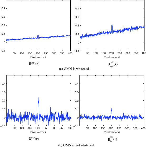
Furthermore, in order to see the effect of noise whitening, Figure 12.6 shows the results of δ^OSP(r) and where the Gaussian–Markov noise with CC = 0.8 was not whitened and also whitened by using the square-root matrix of , analytically (Poor, 1994, p. 60).

As shown in Figure 12.6, the whitening had slight impact on the performance of δ^OSP(r) and in the sense that the abundance fractions of creosote leaves and background signatures were detected more accurately. This was particularly visible for δ^OSP(r). These simple experiments also demonstrated that OSP performance could be improved by a whitening process, but might not be significant. So, the pay-off may not be great given that a reliable estimation of noise covariance may be difficult to obtain.

Figure 12.2 Detection results of δ^OSP(r) in white Gaussian noise and white uniform noise with various SNRs.

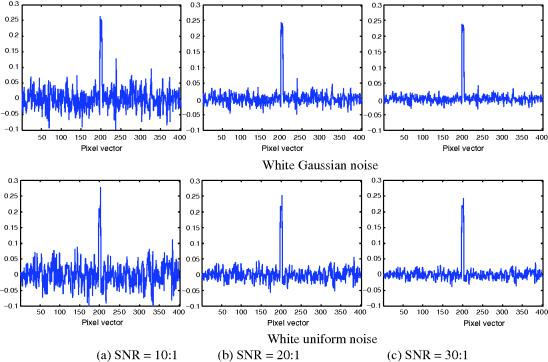
Figure 12.3 Detection results of in white Gaussian noise and white uniform noise with various SNRs.

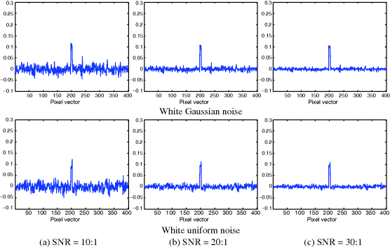
Table 12.1 Detected abundance fractions of “creosote leaves” at 198–202 pixels by δ^OSP(r) and

Figure 12.4 Detection results of δ^OSP(r) in GMN with different correlation coefficients and SNRs.

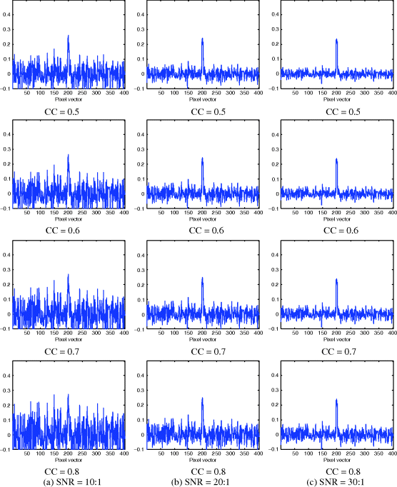
Figure 12.5 Detection results of in GMN with different correlation coefficients and SNRs.

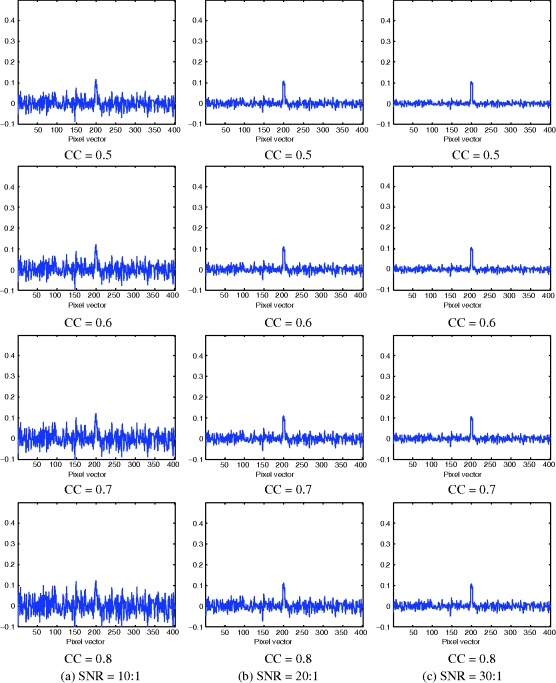
Table 12.2 Detected abundance fractions of “creosote leaves” at 198–202 pixels by δ^OSP(r) and with LSEs.

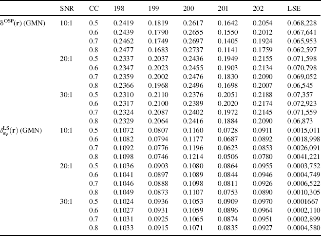
Figure 12.6 Results of δ^OSP(r) and where the GMN with CC = 0.8 with/without being whitened.