8.5 Trees

Search in book...
Toggle Font Controls
Create new playlist

Name your new playlist

Playlist description (optional)
Sign In

Email address

Password

Forgot Password?

or

Continue with Facebook

Continue with Google
Sign Up

Full Name

Email address

Confirm Email Address

Password

or

Continue with Facebook

Continue with Google

8.5 Trees

Abstract structures such as lists, stacks, and queues are linear in nature. Only one relationship in the data is being modeled. Items are next to each other in a list or are next to each other in terms of time in a stack or queue. Depicting more complex relationships requires more complex structures. Take, for example, an animal hierarchy. General classification occurs at higher levels and the labels get more specific as you move down. Each node could have many below it (FIGURE 8.5).

In animal hierarchical structure, the mammals are branched into three as horse, dog, and whale. Further, the dogs are sub-branched into hound and terrier. — FIGURE 8.5 An animal hierarchy forms a tree

Such hierarchical structures are called trees, and there is a rich mathematical theory relating to them. In computing, however, we often restrict our discussion to binary trees. In binary trees, each node in the tree can have no more than two children.

Binary Trees

A binary tree is a tree in which each node is capable of having at most two successor nodes, called children. Each of the children, being nodes in the binary tree, can also have up to two child nodes, and these children can also have up to two children, and so on, giving the tree its branching structure. The beginning of the tree is a unique starting node called the root, which is not the child of any node. FIGURE 8.6 shows a binary tree containing integer values.

Each node in the tree may have zero, one, or two children. The node to the left of a node, if it exists, is called its left child. For example, in Figure 8.6, the left child of the root node contains the value 2. The node to the right of a node, if it exists, is its right child. The right child of the root node in Figure 8.6 contains the value 3. If a node has only one child, the child could be on either side, but it is always on one particular side. In Figure 8.6, the root node is the parent of the nodes containing 2 and 3. If a node in the tree has no children, it is called a leaf. In Figure 8.6, the nodes containing 7, 8, 9, and 10 are leaf nodes.

John von Neumann²

Courtesy of the U.S. Department of Energy

John von Neumann was a brilliant mathematician, physicist, logician, and computer scientist. Legends have been passed down about his astonishing memory and the phenomenal speed at which von Neumann solved problems. He used his talents not only for furthering his mathematical theories, but also for memorizing entire books and reciting them years after he had read them.

John von Neumann was born in Hungary in 1903, the oldest son of a wealthy Jewish banker. He was able to divide 8-digit numbers in his head by the age of 6. He entered high school by the time he was 11, and it wasn’t long before his math teachers recommended he be tutored by university professors. He received his diploma in chemical engineering from the Technische Hochschule in Zürich in 1926. In the same year, he received his doctorate in mathematics from the University of Budapest, with a thesis on set theory.

von Neumann came to the United States in the early 1930s to teach at Princeton, while still keeping his academic posts in Germany. He resigned the German posts when the Nazis came to power; he was not, however, a political refugee as so many were at that time. While at Princeton, he worked with the talented and as-yet-unknown British student Alan Turing. He continued his brilliant mathematical career, becoming editor of Annals of Mathematics and co-editor of Compositio Mathematica. During World War II, von Neumann was hired as a consultant for the U.S. Armed Forces and related civilian agencies because of his knowledge of hydrodynamics. He was also called upon to participate in the construction of the atomic bomb in 1943. It was not surprising that, following this work, President Eisenhower appointed him to the Atomic Energy Commission in 1955.

Even though bombs and their performance fascinated von Neumann for many years, a fortuitous meeting in 1944 with Herbert Goldstine, a pioneer who developed one of the first operational electronic digital computers, introduced the mathematician to computers. von Neumann started working on the stored program concept and concluded that internally storing a program eliminated the hours of tedious labor required to reprogram computers (in those days). He also developed a new computer architecture to perform this storage task. Today’s computers are often referred to as “von Neumann machines” because the architectural principles he described have proven so tremendously successful. Computers have changed a lot over the past 50 years, but the basic architecture designed by von Neumann has persisted.

During the 1950s, von Neumann was a consultant for IBM, where he reviewed proposed and ongoing advanced technology projects. One such project was John Backus’s FORTRAN, which von Neumann reportedly questioned, asking why anyone would want more than one machine language.

In 1957, von Neumann died of bone cancer in Washington, D.C., at the age of 54. Perhaps his work with the atomic bomb resulted in the bone cancer that caused the death of one of the most brilliant and interesting minds of the twentieth century.

In addition to specifying that a node may have up to two children, the definition of a binary tree states that a unique path exists from the root to every other node. In other words, every node (except the root) has a unique (single) parent.

Each of the root node’s children is itself the root of a smaller binary tree, or subtree. In Figure 8.6, the root node’s left child, containing 2, is the root of its left subtree, while the right child, containing 3, is the root of its right subtree. In fact, any node in the tree can be considered the root node of a subtree. The subtree whose root node has the value 2 also includes the nodes with values 4 and 7. These nodes are the descendants of the node containing 2. The descendants of the node containing 3 are the nodes with the values 5, 6, 8, 9, and 10. A node is the ancestor of another node if it is the parent of the node or the parent of some other ancestor of that node. (Yes, this is a recursive definition.) In Figure 8.6, the ancestors of the node with the value 9 are the nodes containing 5, 3, and 1. Obviously, the root of the tree is the ancestor of every other node in the tree.

Binary Search Trees

A tree is analogous to an unordered list. To find an item in the tree, we must examine every node until either we find the one we want or we discover that it isn’t in the tree. A binary search tree is like a sorted list in that there is a semantic ordering in the nodes.

A binary search tree has the shape property of a binary tree; that is, a node in a binary search tree can have zero, one, or two children. In addition, a binary search tree has a semantic property that characterizes the values in the nodes in the tree: The value in any node is greater than the value in any node in its left subtree and less than the value in any node in its right subtree. See FIGURE 8.7.

A figure shows a binary search tree. — FIGURE 8.7 A binary search tree

Searching a Binary Search Tree

Let’s search for the value 18 in the tree shown in Figure 8.7. We compare 18 with 15, the value in the root node. Because 18 is greater than 15, we know that if 18 is in the tree it will be in the right subtree of the root. Note the similarity of this approach to our binary search of a linear structure (discussed in Chapter 7). As in the linear structure, we eliminate a large portion of the data with one comparison.

Next we compare 18 with 17, the value in the root of the right subtree. Because 18 is greater than 17, we know that if 18 is in the tree, it will be in the right subtree of the root. We compare 18 with 19, the value in the root of the right subtree. Because 18 is less than 19, we know that if 18 is in the tree, it will be in the left subtree of the root. We compare 18 with 18, the value in the root of the left subtree, and we have a match.

Now let’s look at what happens when we search for a value that is not in the tree. Let’s look for 4 in Figure 8.7. We compare 4 with 15. Because 4 is less than 15, if 4 is in the tree, it will be in the left subtree of the root. We compare 4 with 7, the value in the root of the left subtree. Because 4 is less than 7, if 4 is in the tree, it will be in 7’s left subtree. We compare 4 with 5. Because 4 is less than 5, if 4 is in the tree, it will be in 5’s left subtree. We compare 4 with 1. Because 4 is greater than 1, if 4 is in the tree, it will be in 1’s right subtree. But 1’s left subtree is empty, so we know that 4 is not in the tree.

In looking at the algorithms that work with trees, we use the following conventions: If current points to a node, info(current) refers to the user’s data in the node, left(current) points to the root of the left subtree of current, and right(current) points to the root of the right subtree of current. null is a special value that means that the pointer points to nothing. Thus, if a pointer contains null, the subtree is empty.

Using this notation, we can now write the search algorithm. We start at the root of the tree and move to the root of successive subtrees until we either find the item we are looking for or we find an empty subtree. The item to be searched for and the root of the tree (subtree) are parameters—the information that the subalgorithm needs to execute.

With each comparison, either we find the item or we cut the tree in half by moving to search in the left subtree or the right subtree. In half? Well, not exactly. The shape of a binary tree is not always well balanced. Clearly, the efficiency of a search in a binary search tree is directly related to the shape of the tree. How does the tree get its shape? The shape of the tree is determined by the order in which items are entered into the tree. Look at FIGURE 8.8. In part (a), the four-level tree is comparatively balanced. The nodes could have been entered in several different orders to get this tree. By comparison, the ten-level tree in part (b) could only have come from the values being entered in order.

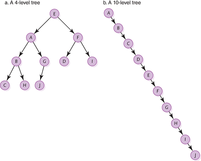
A figure shows two types of binary search trees: 4-level tree and 10-level tree. — FIGURE 8.8 Two variations of a binary search tree

Building a Binary Search Tree

How do we build a binary search tree? One clue lies in the search algorithm we just used. If we follow the search path and do not find the item, we end up at the place where the item would be if it were in the tree. Let’s now build a binary search tree using the following strings: john, phil, lila, kate, becca, judy, june, mari, jim, sue.

Because john is the first value to be inserted, it goes into the root. The second value, phil, is greater than john, so it goes into the root of the right subtree. lila is greater than john but less than phil, so lila goes into the root of the left subtree of phil. The tree now looks like this:

A tree structure starts from “John” roots to the right subtree labeled “phil” that further roots to the left subtree labeled “lila.”

kate is greater than john but less than phil and lila, so kate goes into the root of the left subtree of lila. becca is less than john, so becca goes into the root of the left subtree of john. judy is greater than john but less than phil, lila, and kate, so judy goes into the root of the left subtree of kate. We follow the same path for june as we did for judy. june is greater than judy, so june goes into the root of the right subtree of judy. mari becomes the root of lila’s right subtree; jim becomes the root of the right subtree of becca; and sue becomes the root of the right subtree of phil. The final tree is shown in FIGURE 8.9.

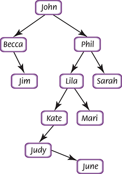
A figure shows a binary search tree with strings. — FIGURE 8.9 A binary search tree built from strings

TABLE 8.1 shows a trace of inserting nell into the tree shown in Figure 8.9. We use the contents of the info part of the node within parentheses to indicate the pointer to the subtree with that value as a root.

Although Put item in tree is abstract, we do not expand it. We would need to know more about the actual implementation of the tree to do so.

Printing the Data in a Binary Search Tree

To print the value in the root, we must first print all the values in its left subtree, which by definition are smaller than the value in the root. Once we print the value in the root, we must print all the values in the root’s right subtree, which by definition are greater than the value in the root. We are then finished. Finished? But what about the values in the left and right subtrees? How do we print them? Why, the same way, of course. They are, after all, just binary search trees.

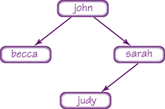
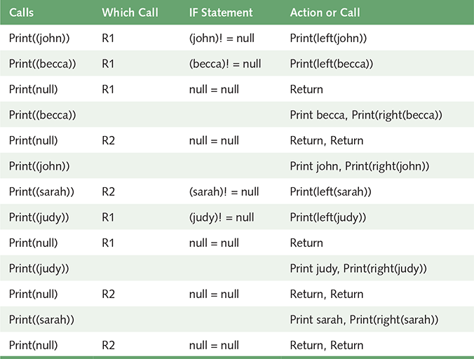
This algorithm sounds too easy. That’s the beauty of recursive algorithms: They are often short and elegant (although sometimes they take some thought to trace). Let’s write and trace this algorithm using the tree shown below the algorithm. We number the calls in our trace because there are two recursive calls. See TABLE 8.2.

A tree starts from “john” that roots to a left subtree labeled “becca” and right subtree labeled “sarah.” The sarah further roots to the left subtree labeled “judy.”

This algorithm prints the items in the binary search tree in ascending value order. Other traversals of the tree print the items in other orders. We explore them in the exercises.

Other Operations

At this point you may have realized that a binary search tree is an object with the same functionality as a list. The characteristic that separates a binary search tree from a simple list is the efficiency of the operations; the other behaviors are the same. We have not shown the Remove algorithm, because it is too complex for this text. We have also ignored the concept length, which must accompany the tree if it is to be used to implement a list. Rather than keep track of the number of items in the tree as we build it, let’s write an algorithm that counts the number of nodes in the tree.

How many nodes are in an empty tree? Zero. How many nodes are in any tree? There are one plus the number of nodes in the left subtree and the number of nodes in the right subtree. This definition leads to a recursive definition of the Length operation:

..................Content has been hidden....................

You can't read the all page of ebook, please click here login for view all page.

IF (tree is NOT null)
Print(left(tree))	// Recursive call R1
Write info(tree)
Print(right(tree))	// Recursive call R2

Table of Contents for 8.5 Trees

Create new playlist

Sign In

Sign Up

Table of Contents for
8.5 Trees