
11.5. Dose-Finding Procedures
As was indicated in Section 11.1, once a positive dose-response has been established, clinical researchers are interested in determining the optimal dose range for their experimental drug known as the therapeutic window. As an example, the usual adult dosage range for prescription ibuprofen is 200 to 800 mg three or four times per day, not to exceed 3200 mg total daily. In other words, ibuprofen's therapeutic window extends from 600 mg to 3200 mg per day. The therapeutic window is more conservative for over-the-counter (OTC) versions. The usual adult dosage range for OTC ibuprofen is 200 to 400 mg every four to six hours, not to exceed 1200 mg total daily.
The therapeutic window is defined by the minimum effective dose (MED) and maximum tolerated dose (MTD). As the name implies, the MED is chosen to ensure the efficacy of both it and all dose levels higher than it (up to the upper limit of the therapeutic window). Likewise, as the maximum dose, an MTD is chosen to ensure the safety of both it and all dose levels lower than it. In the drug approval process, safety (including the determination of the MTD) is frequently assessed through simple comparisons of adverse events across treatment arms. The Center for Drug Evaluation and Research at the FDA is currently studying how to provide a more detailed statistical assessment of the safety profile of a drug by taking into account the time course or other important factors.
In this section, we will concentrate on the statistical determination of the MED in dose-ranging studies with a placebo control, given that a safe range of doses has been tentatively determined. For more information on simultaneous tests for identifying the MED and MTD, see Bauer, Brannath and Posch (2001) and Tamhane and Logan (2002). Further, Bauer et al (1998) describe testing strategies for dose-ranging studies with both negative and positive controls.
11.5.1. MED Estimation under the Monotonicity Assumption
The problem of estimating the MED is often stated as a problem of stepwise multiple testing. Clinical researchers begin with the highest dose or the dose corresponding to the largest treatment difference and proceed in a stepwise fashion until they encounter a non-significant treatment difference. The immediately preceeding dose is defined as the minimum effective dose (MED).
To simplify the statement of the multiple testing problem arising in the MED estimation, it is common to make the following two assumptions known as the monotonicity constraints:
All doses are no worse than placebo.
If Dose k is not efficacious, the lower doses (Doses 1 through k − 1) are not efficacious either.
These assumptions are reasonable in clinical trials with a positive dose-response relationship. However, they are not met when the true dose-response function is umbrella-shaped and stepwise tests relying on the monotonicity assumptions break down in the presence of non-monotone dose-response curves.
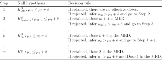
Under the monotonicity constraints, the MED estimation problem is easily expressed in terms of sequential testing of m null hypotheses associated with the m dose levels. To define the null hypotheses, assume that the drug's effect is expressed as a positive shift. Further, the observations, yij, are assumed to be normally distributed and follow an ANOVA model
where μ0,...,μm are the true treatment means in the placebo and m dose groups and εij's are residuals. Given this model, the null hypotheses used in MED estimation are displayed in Table 11.3. The clinically important difference is denoted by δ. When the clinically important difference is assumed to be 0, the kth null hypothesis, HM0k, simplifies to
The first null hypothesis in Table 11.3, HM01, states that Dose 1 is ineffective and therefore its rejection implies that Dose 1 is the MED. Likewise, if HM01 is retained but HM02 is rejected, Dose 2 is declared the MED, etc.
| Null hypothesis | Interpretation |
|---|---|
| HM01 : μ0 ≤ μ1 < μ0 + δ | Dose 1 is ineffective |
| HM02 : μ0 ≤ μ1,μ2 < μ0 + δ | Doses 1 and 2 are ineffective |
| ⋮ | ⋮ |
| HM0k : μ0 ≤ μ1,...,μk < μ0 + δ | Doses 1,...,k are ineffective |
| ⋮ | ⋮ |
| HM0m : μ0 ≤ μ1,...,μm < μ0 + δ | All doses are ineffective |
The stepwise testing approach goes back to early work by Tukey, Ciminera and Heyse (1985), Mukerjee, Robertson and Wright (1987), Ruberg (1989) and others who proposed multiple-contrast methods for examining dose-related trends. This section focuses on stepwise contrast tests considered by Tamhane, Hochberg and Dunnett (1996) and Dunnett and Tamhane (1998). We can also construct stepwise testing procedures for estimating the MED using other tests, e.g., isotonic tests described in Section 11.3. For more information about MED estimation procedures based on the Williams test, see Dunnett and Tamhane (1998) and Westfall et all (1999, Section 8.5.3).
11.5.2. Multiple-Contrast Tests
The null hypotheses displayed in Table 11.3 will be tested using multiple-contrast tests. It is important to understand the difference between multiple-contrast tests introduced here and the tests discussed in Section 11.3 (known as single-contrast tests). As their name implies, single-contrast tests rely on a single contrast and are used mainly for studying the overall drug effect. Each of multiple-contrast tests discussed in this subsection actually relies on a family of contrasts
These contrasts are applied in a stepwise manner to test HM01,...,HM0m. The k null hypothesis, HM0k, is tested using the following t statistic
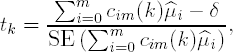
where ![]() 0,...,
0,...,![]() m are the sample treatment means in the placebo and m dose groups. Assuming n patients in each treatment group, each of the t statistics follows a t distribution with ν = (m + 1)(n − 1) degrees of freedom.
m are the sample treatment means in the placebo and m dose groups. Assuming n patients in each treatment group, each of the t statistics follows a t distribution with ν = (m + 1)(n − 1) degrees of freedom.
It is important to note that the contrasts can be constructed on any scale when the clinically significant difference (δ) is 0. The contrast coefficients are automatically standardized when the test statistic is computed. However, when δ > 0, the contrasts need to be on the correct scale because the standardization occurs only after δ is subtracted. To ensure the correct scale is used, the contrast coefficients are defined in such a way that c0m(k) is negative, ckm(k) is positive and the positive coefficients add up to 1.
Popular multiple-contrast tests used in dose-finding are defined below.
11.5.2.1. Pairwise Contrasts
The easiest way to compare multiple dose groups to placebo is by considering all possible dose-placebo comparisons. The associated test is based on a family of pairwise contrasts. The following coefficients are used when the Dose k is compared to placebo:
and all other coefficients are equal to 0.
11.5.2.2. Helmert Contrasts
Unlike the pairwise contrast, the Helmert test combines information across several dose groups. Specifically, when comparing Dose k to placebo, this test assumes that the lower doses (Doses 1 through k − 1) are not effective and pools them with placebo. The kth Helmert contrast is defined as follows:
The other coefficients are equal to 0. Helmert contrasts are most powerful when the lower doses are similar to placebo.
11.5.2.3. Reverse Helmert Contrasts
The reverse Helmert contrast test is conceptually similar to the regular Helmert test but it does everything the other way around. The reverse Helmert test combines information across doses by assuming that the lower doses are as effective as Dose k. Thus, the kth reverse Helmert contrast are given by
The remaining coefficients are equal to 0. Reverse Helmert contrasts are most powerful when the treatment effect quickly plateaus and the larger doses are similar to the highest dose.
11.5.2.4. Linear Contrasts
The linear contrast test assigns weights to the individual doses that increase in a linear fashion. Dose k is compared to placebo using the following contrast:

where

and [k/2] is the largest integer in k/2. As before, the other coefficients are equal to 0. Linear contrasts are most powerful when the MED is near the middle of the range of doses tested in a trial.
Put simply, the Helmert, reverse Helmert and linear contrasts each correspond to different shapes of the dose-response curve for which they are most powerful. Figure 11.6 displays the treatment effect configurations that lead to the maximum expected value of the t statistic for each type of contrast.
Figure 11-6. Treatment effect configurations leading to the maximum expected value of the t statistic under the monotonicity constraint

11.5.3. Closed Testing Procedures Based on Multiple Contrasts
In this section, we will consider the MED estimation problem from a multiple testing perspective and focus on MED estimation procedures that control the overall Type I error rate. As was pointed out in the Introduction, the control of the Type I error probability is required in registration trials and is less common in Phase II trials.
Two general stepwise procedures for testing HM01,...,HM0m can be constructed based on the principle of closed testing proposed by Marcus, Peritz and Gabriel (1976). The principle has provided a foundation for numerous multiple tests and has found a large number of applications in multiplicity problems arising in clinical trials. For example, Kodell and Chen (1991) and Rom, Costello and Connell (1994) applied the closed testing principle to construct multiple tests for dose-ranging studies.
Very briefly, the closed testing principle is based on a hierarchical representation of a multiplicity problem. In general, we need to consider all possible intersections of the null hypotheses of interest (known as a closed family of hypotheses) and test each intersection at the same significance level. After that the results need to be combined to make inferences about the original null hypotheses. In this case, the family of null hypotheses defined in Table 11.3 is already a closed family and therefore closed testing procedures have a simple sequentially rejective form.
Two closed procedures for estimating the MED are introduced below. The first procedure begins with the most significant dose-placebo comparison and then works downward. For this reason, this procedure is known as the step-down procedure. Note that the idea behind the step-down approach is that the order in which the dose-placebo tests are examined is driven by the data. By contrast, the fixed-sequence procedure requires that the tasting sequence be specified prior to data analysis.
11.5.4. Step-Down MED Estimation Procedure
Consider the m contrast test statistics, t1,...,tm, and order them from the most significant to the least significant. The ordered t statistics will be denoted by
The step-down MED estimation procedure is defined below:
Consider the most significant t statistic, t(1), and compare it to the prespecified critical value (e.g., two-sided 0.05 critical value) derived from the null distribution of t1,..., tm with ν = (m + 1)(n − 1) degrees of freedom and correlation matrix ρ. This critical value is denoted by c1. If t(1) exceeds c1, the corresponding null hypothesis is rejected and one proceeds to the second most significant t statistic.
The next statistic, t(2), is compared to c2 which is computed from the null distribution of t1,..., tm−1 with the same number of degrees of freedom and correlation matrix as above (c2 is less than c1). If t(2) > c2, reject the corresponding null hypothesis and examine t(3), etc.
The step-down procedure terminates as soon as it encounters a null hypothesis which cannot be rejected.
Let l be the index of the lowest dose which is significantly different from placebo. When testing stops, the monotonicity assumption implies that the null hypotheses HM0l,...,HM0m should be rejected and therefore Dose l is declared the MED.
11.5.5. Fixed-Sequence MED Estimation Procedure
This procedure relies on the assumption that the order in which the null hypotheses are tested is predetermined. Let t[1],..., t[m] denote the a priori ordered t contrast statistics (any ordering can be used as long as it is prespecified). The fixed-sequence procedure is defined as follows:
Compare t[1] to the prespecified critical value of the t distribution with ν degrees of freedom (denoted by c). If t[1] is greater than c, the corresponding null hypothesis is rejected and the next test statistic is examined.
The next test statistic, t[2], is also compared to c and the fixed-sequence procedure proceeds in this manner until it fails to reject a null hypothesis.
The dose corresponding to the last rejected null hypothesis is declared the MED.
The step-down and fixed-sequence procedures protect the Type I error rate with respect to the entire family of null hypotheses shown in Table 11.3 given the monotonicity constraints. To be more precise, the two procedures control the probability of erroneously rejecting any true null hypothesis in the family regardless of which and how many other null hypotheses are true. This is known as the control of the familywise error rate in the strong sense.
11.5.6. Pairwise Multiple-Contrast Test in the Hypertension Trial
To illustrate the use of stepwise tests in MED estimation, we will begin with the pairwise contrast test. Unlike other contrast tests, the pairwise test is easy to implement in practice because the associated correlation matrix has a very simple structure. In the balanced case, the correlation between any two pairwise t statistics is 0.5 and, due to this property, we can carry out the pairwise contrast test by a stepwise application of the well-known Dunnett test.
In what follows, we will apply the step-down and fixed-sequence versions of the Dunnett test to find the MED in the hypertension trial. First, Program 11.8 assesses the overall drug effect in the hypertension trial using the three contrast tests defined in Section 11.3.
Example 11-8. Contrast tests in the hypertension trial
proc mixed data=hypertension;
    ods select contrasts;
    class dose;
    model change=dose;
    contrast "Linear" dose −3 −1 1 3;
    contrast "Modified linear" dose −12 −2 2 12;
    contrast "Maximin" dose −0.866 −0.134 0.134 0.866;
run; |
Example. Output from Program 11.8
Contrasts

                    Num     Den
Label                DF      DF    F Value    Pr > F

Linear                1      64       8.61    0.0046
Modified linear       1      64       7.70    0.0072
Maximin 1 64 7.62 0.0075 |
Output 11.8 shows the test statistics and p-values of the linear, modified linear and maximin tests. All three p-values are very small which indicates that the response improves in a highly significant manner with increasing dose in the hypertension trial.
Now that a positive dose-response relationship has been established, we are ready for a dose finding exercise. First, we will use the step-down version of the Dunnett test and after than apply the fixed-sequence Dunnett test.
11.5.7. Step-Down Dunnett Test in the Hypertension Trial
Program 11.9 carries out the step-down Dunnett test to determine the MED in the hypertension trial with the clinically important difference δ = 0. The program uses PROC MIXED to compute the t statistics associated with the three dose-placebo comparisons. The statistics are ordered from the most significant to the least significant and compared to successively lower critical values. Specifically, the critical values of the step-down procedure are computed from the Dunnett distribution for the case of three, two and one dose-placebo comparisons. These critical values are found using the PROBMC function. Note that the PROBMC function assumes a balanced case. Therefore we computed the average number of patients per group in the hypertension trial (17) and plugged the number into the well-known formula for calculating degrees of freedom (4(17−1)=64).
Example 11-9. Step-down Dunnett test in the hypertension trial
ods listing close;
* Compute t statistics for three dose-placebo comparisons;
proc mixed data=hypertension;
    class dose;
    model change=dose;
    lsmeans dose/pdiff adjust=dunnett;
    ods output diffs=dunnett;
* Order t statistics;
proc sort data=dunnett;
    by descending tvalue;
* Compute critical values (based on Dunnett distribution);
data critical;
    set dunnett nobs=m;
    format c 5.2;
    order=_n_;
    c=probmc("DUNNETT2",.,0.95,64,m-_n_+1);
    label c='Critical value';
proc print data=critical noobs label;
    var order dose tvalue c;
    ods listing;
run; |
Example. Output from Program 11.9
Critical order dose t Value value 1 20 2.80 2.41 2 40 2.54 2.26 3 10 1.10 2.00 |
Output 11.9 shows the t statistics computed in the hypertension trial and associated critical values of the step-down Dunnett test. The dose groups are ordered by their t statistic and the ORDER variable shows the order in which the doses will be compared to placebo. The following algorithm is used to determine significance of the t statistics listed in Output 11.9.
The most significant test statistic (t(1) = 2.80) arises when we compare the medium dose to placebo. This statistic is greater than the critical value (c1 = 2.41) and therefore we proceed to the next dose-placebo comparison.
The test statistic for the high dose vs. placebo comparison (t(2) = 2.54) also exceeds the corresponding critical value (c2 = 2.26). Due to this significant result, we will now compare the low dose versus placebo.
Examining the last dose-placebo comparison, we see that the test statistic (t(3) = 1.10) is less than c3 = 2.00.
Since the last dose-placebo comparison did not yield a significant result, the medium dose (20 mg/day) is declared the MED. The multiple comparisons summarized in Output 11.9 enable clinical researchers to provide the following characterization of the dose-response function in the hypertension trial. First, as was shown in Output 11.8, the overall dose-response trend in diastolic blood pressure change is positive and highly significant. Further, we have concluded from Output 11.9 that the 20 mg/day dose is the MED and thus the positive dose-response trend in the hypertension trial is due to statistically significant treatment differences at the 20 mg/day and 40 mg/day dose levels.
It is important to remember that the step-down testing approach relies heavily on the monotonicity assumption. When this assumption is not met, the approach may lead to results that look counterintuitive. Suppose, for example, that we conclude significance for the low and medium doses but not for the high dose. In this case, the low dose is declared the MED even though we did not actually reject the null hypothesis of no drug effect at the high dose.
11.5.8. Fixed-Sequence Pairwise Test in the Hypertension Trial
Program 11.10 takes a different approach to the dose-finding problem in the hypertension trial. It identifies the MED using the fixed-sequence version of the Dunnett test. To understand the difference between the two approaches, recall that the step-down procedure (see Output 11.9) compares ordered t statistics to successively lower Dunnett critical values whereas the fixed-sequence procedure compares the same t statistics to a constant critical value derived from a t distribution (it is the two-sided 95th percentile of the t distribution with 64 degrees of freedom). Additionally, the fixed-sequence procedure requires that the three tests for individual dose-placebo comparisons be ordered before the dose finding exercise begins. We will assume a natural testing sequence here: high dose vs. placebo, medium dose vs. placebo and low dose vs. placebo.
Example 11-10. Fixed-sequence pairwise test in the hypertension trial
ods listing close;
* Compute t statistics for three dose-placebo comparisons;
proc mixed data=hypertension;
    class dose;
    model change=dose;
    lsmeans dose/pdiff adjust=dunnett;
    ods output diffs=dunnett;
* Prespecified testing sequence;
data dunnett;
    set dunnett;
    if dose=10 then order=3;
    if dose=20 then order=2;
    if dose=40 then order=1;
* Order t statistics;
proc sort data=dunnett;
    by order;
* Compute critical values (based on t distribution);
data critical;
    set dunnett;
    format c 5.2;
    c=tinv(0.975,64);
    label c='Critical value';
proc print data=critical noobs label;
    var order dose tvalue c;
    ods listing;
run; |
Example. Output from Program 11.10
Critical order dose t Value value 1 40 2.54 2.00 2 20 2.80 2.00 3 10 1.10 2.00 |
Output 11.10 lists t statistics for the three dose-placebo comparisons and critical values of the fixed-sequence procedure. Note that the testing sequence is no longer data-driven—the doses are ordered according to the prespecified rule (the ORDER variable indicates the order in which the doses will be compared to placebo). Also, the critical values in Output 11.10 are uniformly smaller than those shown in Output 11.9 with the exception of the low dose vs. placebo test. This means that the fixed-sequence dose-finding procedure is likely to find more significant differences than the step-down procedure provided the prespecified testing sequence is consistent with the true dose-response curve.
Proceeding in a stepwise fashion, we see that the tests statistics associated with the two highest doses (2.54 and 2.80) are greater than the critical value. However, the low dose is not significantly different from placebo because its t statistic is too small. Given this configuration of t values, we conclude that the medium dose (20 mg/day dose) is the MED. When we compare this to Output 11.9, it is easy to see that the two MED estimation procedures resulted in the same minimally effective dose. However, the conclusions are not guaranteed to be the same, especially when the dose-response curve is not perfectly monotone.
11.5.9. Other Multiple-Contrast Tests in the Hypertension Trial
The dose-finding procedures described so far relied on pairwise comparisons. Intuitively, these procedures are likely to be inferior (in terms of power) to procedures that pool information across dose levels. For example, consider procedures based on a stepwise application of the Helmert or linear contrasts. In general, the problem of computing critical values for the joint distribution of t statistics in stepwise procedures presents a serious computational challenge, especially in the case of unequal sample sizes. This is due to the complex structure of associated correlation matrices. Although exact numerical methods have been discussed in the literature (see, for example, Genz and Bretz, 1999), simulation-based approaches are generally more flexible and attractive in practice. Here we will consider a simulation-based solution proposed by Westfall (1997).
Westfall (1997) proposed a Monte Carlo method that can be used in dose-finding procedures based on non-pairwise contrasts. Instead of computing critical values for t statistics as was done in Program 11.9, the Monte Carlo algorithm generates adjusted p-values. The adjusted p-values are then compared to a prespecified significance level (e.g., two-sided 0.05 level) to test the null hypotheses listed in Table 11.3. The algorithm is implemented in the %SimTests macro described in Westfall et al (1999, Section 8.6).[]
[] As this book was going to press, the methods in the %SimTests and %SimIntervals macros were being completely hardcoded in the GLIMMIX procedure in SAS/STAT software. The methodology is described in Westfall and Tobias (2006).
Program 11.11 calls the %SimTests macro to carry out the reverse Helmert multiple-contrast test in the hypertension trial. Reverse Helmert contrasts were chosen because they perform well in clinical trials in which the treatment effect reaches a plateau and other multiple-contrast tests can be used if a different dose-relationship is expected.
As shown in the program, to invoke the %SimTests macro, we need to define several parameters, including the family of reverse Helmert contrasts, the treatment means in the hypertension trial and their covariance matrix. The parameters are specified in the %Estimates and %Contrasts macros using the SAS/IML syntax. Once these parameters have been defined, the macro approximates adjusted two-sided p-values for the three dose-placebo tests using 100,000 simulations.
Example 11-11. Reverse Helmert multiple-contrast test in the hypertension trial
ods listing close;
* Compute treatment means and covariance matrix;
proc mixed data=hypertension;
    class dose;
    model change=dose;
    lsmeans dose/cov;
    ods output lsmeans=lsmeans;
    run;
%macro Estimates;
    use lsmeans;
    * Treatment means;
    read all var {estimate} into estpar;
    * Covariance matrix;
    read all var {cov1 cov2 cov3 cov4} into cov;
    * Degrees of freedom;
    read point 1 var {df} into df;
%mend;
%macro Contrasts;
    * Reverse Helmert contrasts;
    c={1 −1 0 0, 1 −0.5 −0.5 0, 1 −0.3333 −0.3333 −0.3334};
    c=c';
    * Labels;
    clab={"Dose 1 vs Placebo", "Dose 2 vs Placebo", "Dose 3 vs Placebo"};
%mend;
* Compute two-sided p-values using 100,000 simulations;
%SimTests(nsamp=100000,seed=4533,type=LOGICAL,side=B);
proc print data=SimTestOut noobs label;
    var contrast adjp seadjp;
    format adjp seadjp 6.4;
    ods listing;
run; |
Example. Output from Program 11.11
SEAdj
    Contrast          AdjP      P

Dose 1 vs Placebo    0.2753   0.0000
Dose 2 vs Placebo    0.0425   0.0002
Dose 3 vs Placebo 0.0200 0.0002 |
Output 11.11 lists Monte Carlo approximations to the adjusted p-values for the three dose-placebo comparisons as well as associated standard errors. The standard errors are quite small which indicates that the approximations are reliable. Comparing the computed p-values to the 0.05 threshold, we see that the highest two doses are significantly different from placebo whereas the low dose not separate from placebo. As a consequence, the medium dose (20 mg/day dose) is declared the MED. This conclusion is consistent with the conclusions we reached when applying the pairwise multiple-contrast test.
11.5.10. Limitations of Tests Based on the Monotonicity Assumption
It is important to remember that the dose-finding procedures described in the previous subsection control the Type I error rate only if the true dose-response relationship is monotone. When the assumption of a monotonically increasing dose-response relationship is not met, the use of multiple-contrast tests can result in a severely inflated probability of false-positive outcomes (Bauer, 1997; Bretz, Hothorn and Hsu, 2003). This phenomenon will be illustrated below.
Non-monotone dose-response shapes, known as the U-shaped or umbrella-shaped curves, are characterized by a lower response at higher doses (see, for example, Figure 11.1). When the dose-response function is umbrella-shaped and the true treatment difference at the highest dose is not clinically meaningful (i.e., μm − μ0 < δ), the highest dose should not be declared effective. However, if the remaining portion of the dose-response function is monotone, some reasonable tests that control the Type I error rate under the monotonicity constraint may end up declaring the highest dose effective with a very high probability.
11.5.11. Hypothetical Dose-Ranging Trial Example
To illustrate, consider a hypothetical trial in which five doses of an experimental drug are compared to placebo. Table 11.4 shows the true treatment means μ0, μ1, μ2, μ3, μ4 and μ5 as well as true standard deviation σ (the standard deviation is chosen in such a way that σ/√n = 1). Assume that the clinically important treatment difference δ is 0.
| Treatment group | ||||||
|---|---|---|---|---|---|---|
| Placebo | Group 1 | Group 2 | Group 3 | Group 4 | Group 5 | |
| n | 5 | 5 | 5 | 5 | 5 | 5 |
| Mean | 0 | 0 | 0 | 2.5 | 5 | 0 |
| SD | 2.236 | 2.236 | 2.236 | 2.236 | 2.236 | 2.236 |
It can be shown that the sequential test based on pairwise contrasts (i.e., stepwise Dunnett test) controls the familywise error rate under any configuration of true treatment means. However, when other contrast tests are carried out, the familywise error rate becomes dependent on the true dose-response shape and can become considerably inflated when an umbrella-shaped dose-response function (similar to the one shown in Table 11.4) is encountered.
Consider, for example, the linear contrast test. If linear contrasts are used for detecting the MED in this hypothetical trial, the probability of declaring Dose 5 efficacious will be 0.651 (using a t test with 24 error degrees of freedom). To see why the linear contrast test does not control the Type I error rate, recall that, in testing HM05 defined in Table 11.3, positive weights are assigned to the treatment differences ![]() 4 −
4 − ![]() 1 and
1 and ![]() 3 −
3 − ![]() 2. The expected value of the numerator of the t-statistic for testing H05 is given by
2. The expected value of the numerator of the t-statistic for testing H05 is given by

As a result, the test statistic has a non-central t distribution with a positive non-centrality parameter and thus the linear contrast test will reject the null hypothesis HM05 more often than it should.
The reverse Helmert contrast test, like the linear contrast test, can also have too high an error rate when the true dose-response curve is umbrella-shaped. In the hypothetical trial example, the probability of declaring the highest dose efficacious will be 0.377 (again, based on a t test with 24 degrees of freedom). This error rate is clearly much higher than 0.05. Combining the signal from the third and fourth doses into the estimate ![]() 5 causes the reverse Helmert contrast test to reject too often.
5 causes the reverse Helmert contrast test to reject too often.
The regular Helmert contrast test does control the Type I error rate in studies with umbrella-shaped dose-response curves. However, it can have an inflated Type I error rate under other configurations. In particular, the Type I error probability can be inflated if the response at lower doses is worse than the response observed in the placebo group. Figure 11.7 shows the general shapes of treatment effect configurations that can lead to inflated Type I error rates for each type of contrast.
Figure 11-7. Treatment effect configurations that can lead to inflated Type I error rates

The choice of which contrast test to use in dose-finding problems is thus clear:
If a monotonically increasing dose-response relationship can be assumed, clinical researchers need to choose contrasts according to which dose-response shape in Figure 11.6 is expected.
If a monotone dose-response relationship cannot be assumed, one must choose pairwise contrasts to protect the overall Type I error probability.
11.5.12. MED Estimation in the General Case
In this section we will discuss a dose-finding approach that does not rely on the assumption of a monotone dose-response relationship.
The closed testing principle is widely used in a dose-ranging setting to generate stepwise tests for determining optimal doses. Here we will focus on applications of another powerful principle known as the partitioning principle to dose finding. The advantage of the partitioning principle is two-fold. First, as shown by Finner and Strassberger (2002), the partitioning principle can generate multiple tests at least as powerful as closed tests. Secondly, the partitioning principle makes drawing statistical inferences relatively clear-cut: the statistical inference given is simply what is consistent with the null hypotheses which have not been rejected (Stefansson, Kim and Hsu, 1988; Hsu and Berger, 1999).
The partitioning principle is based on partitioning the entire parameter space into disjoint null hypotheses which correspond to useful scientific hypotheses to be proved. Since these null hypotheses are disjoint, exactly one of them is true. Therefore, testing each null hypothesis at a prespecified α level, e.g., α = 0.05, controls the familywise error rate in the strong sense without any multiplicity adjustments.
To demonstrate how the partitioning principle can be used in dose finding, consider the dose-ranging study introduced earlier in this section. This study is conducted to test m doses of a drug versus placebo. Assume that positive changes in the response variable correspond to a beneficial effect. Table 11.5 shows a set of partitioning hypotheses that can be used in finding the MED.

|
It is easy to check that the null hypotheses displayed in Table 11.5 are mutually exclusive and only one of them can be true. For example, if HP0m is true (Dose m is ineffective), HP0k (Doses k + 1,...,m are effective but Dose k is ineffective) must be false. Because of this interesting property, testing each null hypothesis at a prespecified α level controls the familywise error rate in the strong sense at the α level. Note that the last hypothesis, HP00, does not really need to be tested to determine which doses are effective; however, it is useful toward pivoting the tests to obtain a confidence set. Secondly, the union of the hypotheses is the entire parameter space and thus inferences resulting from testing these hypotheses are valid without any prior assumption on the shape of the dose-response curve.
As the null hypotheses listed in Table 11.5 partition the entire parameter space, drawing useful inferences from testing HP01,...,HP0m is relatively straightforward. We merely states the inference which is logically consistent with the null hypotheses that have not been rejected. Consider, for example, the hypertension trial in which four doses were tested against placebo (m = 4). The union of HP04 (Dose 4 is ineffective) and HP03 (Dose 4 is effective but Dose 3 is ineffective) is "either Dose 3 or Dose 4 is ineffective." Thus, the rejection of HP03 and HP04 implies that both Dose 3 and Dose 4 are effective.
In general, if HP0k,...,HP0m are rejected, we conclude that Doses k, ..., m are all efficacious because the remaining null hypotheses in Table 11.5, namely, HP01,...,HP0(k-1) are consistent with this inference. As a consequence, Dose k is declared the MED.
11.5.13. Shortcut Testing Procedure
The arguments presented in the previous section lead to a useful shortcut procedure for determining the MED in dose-ranging trials. The shortcut procedure is defined in Table 11.6.
|
The dose-finding procedure presented in Table 11.6 is equivalent to the fixed-sequence procedure based on pairwise comparisons of individual doses to placebo (see Section 11.5.6). The SAS code for implementing this procedure can be found in Program 11.10.
It is important to remember that the parameter space should be partitioned in such a way that dose levels expected to show a greater response are tested first and the set of dose levels inferred to be efficacious is contiguous. For example, suppose that the dose-response function in a study with four active doses is expected to be umbrella-shaped. In this case we might partition the parameter space so that dose levels are tested in the following sequence: Dose 3, Dose 4, Dose 2 and Dose 1. However, it is critical to correctly specify the treatment sequence. It is shown in Bretz, Hothorn and Hsu (2003) that the shortcut procedure that begins at the highest dose suffers a significant loss of power when the dose-response function is not monotone.
11.5.14. Simultaneous Confidence Intervals
Another important advantage of using the partitioning approach is that, unlike closed testing procedures, partitioning procedures are easily inverted to derive simultaneous confidence intervals for the true treatment means or proportions. For example, Hsu and Berger (1999) demonstrated how partitioning-based simultaneous confidence sets can be constructed for multiple comparisons of dose groups to a common control.
To define the Hsu-Berger procedure for computing stepwise confidence intervals, consider the ANOVA model introduced in the beginning of Section 11.5 and let
be the lower limit of the naive one-sided confidence interval for μk-μ0. Here s is the pooled sample standard deviation and tα,ν is the upper 100αth percentile of the t distribution with ν = 2(n − 1) degrees of freedom and n is the number of patients per group. The naive limits are not adequate in the problem of multiple dose-placebo comparisons because their simultaneous coverage probability is less than its nominal value, 100(1 − α)%. To achieve the nominal coverage probability, the confidence limits l1,...,lm need to be adjusted downward. The adjusted lower limit for the true treatment difference μk − μ0 will be denoted by l*k.
Assume that the doses will be compared with placebo beginning with Dose m, i.e., Dose m vs. placebo, Dose m − 1 vs. placebo, etc. As before, any other testing sequence can be used as long as it is not data-driven. A family of one-sided stepwise confidence intervals with a 100(1 − α)% coverage probability is defined in Table 11.7.
Program 11.12 uses the Hsu-Berger method to compute one-sided confidence intervals with a simultaneous 95% coverage probability for the treatment means in the hypertension study[]. As in Program 11.10, we will consider a testing sequence that begins at the high dose (high dose vs. placebo, medium dose vs. placebo and low dose vs. placebo). Also, the clinically important reduction in diastolic blood pressure will be set to 0 (δ=0).
[] Program 11.12 is based on SAS code published in Dmitrienko et al (2005, Section 2.4).
Example 11-12. Simultaneous confidence intervals in the hypertension trial
ods listing close;
* Compute mean squared error;
proc glm data=hypertension;
    class dose;
    model change=dose;
    ods output FitStatistics=mse(keep=rootmse);
* Compute n and treatment mean in placebo group;
proc means data=hypertension;
    where dose=0;
    var change;
    output out=placebo(keep=n1 mean1) n=n1 mean=mean1;
* Compute n and treatment mean in dose groups;
proc means data=hypertension;
    where dose>0;
    class dose;
    var change;
    output out=dose(where=(dose^=.)) n=n2 mean=mean2;
* Prespecified testing sequence;
data dose;
    set dose;
    if _n_=1 then set mse;
    if _n_=1 then set placebo;
    if dose=10 then order=3;
    if dose=20 then order=2;
    if dose=40 then order=1;
* Order doses;
proc sort data=dose;
    by order;
data dose;
set dose;
retain reject 1;
format lower adjlower 5.2;
delta=0;
lower=mean2-mean1-tinv(0.95,n1+n2-2)*sqrt(1/n1+1/n2)*rootmse;
if reject=0 then adjlower=.;
if reject=1 and lower>delta then adjlower=delta;
if reject=1 and lower<=delta then do; adjlower=lower; reject=0; end;
label lower='Naive 95% lower limit'
adjlower='Adjusted 95% lower limit';
proc print data=dose noobs label;
var order dose lower adjlower;
ods listing;
run; |
Example. Output from Program 11.12
Naive 95%    Adjusted
                   lower      95% lower
order    dose      limit        limit

  1       40        1.82         0.00
  2       20        2.33         0.00
3 10 −1.26 −1.26 |
Output 11.12 displays the naive and adjusted confidence limits for the mean reduction in diastolic blood pressure in the three dose groups compared to placebo as well as the order in which the doses are compared to placebo (ORDER variable). As was explained above, adjusted limits that result in a confidence region with a 95% coverage probability are computed in a stepwise manner. The lower limits of the naive one-sided confidence interval for the high and medium doses are greater than the clinically important difference δ=0 and thus the corresponding adjusted limits are set to 0. The mean treatment difference between the low dose and placebo is not significant (the naive confidence interval contains 0) and therefore the adjusted limit is equal to the naive limit. If the hypertension trial included more inefficient dose groups, the adjusted confidence limits for those doses would remain undefined.