Linear regression belongs to the family of regression algorithms. The goal of regression is to find relationships and dependencies between variables. It is modeling the relationship between a continuous scalar dependent variable y (also, label or target in machine learning terminology) and one or more (a D-dimensional vector) explanatory variables (also, independent variables, input variables, features, observed data, observations, attributes, dimensions, data point, and so on) denoted x using a linear function. In regression analysis, the goal is to predict a continuous target variable, as shown in the following figure:
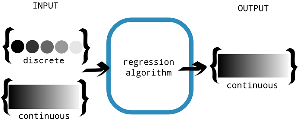
discrete or continuous (source: Nishant Shukla, Machine Learning with TensorFlow, Manning Publications co. 2017)
Now, you might have some confusion in your mind about what the basic difference between a classification and a regression problem is. The following information box will make it clearer:
The model for a multiple regression that involves a linear combination of input variables takes the following form:
y = ss0 + ss1x1 + ss2x2 + ss3x3 +..... + e
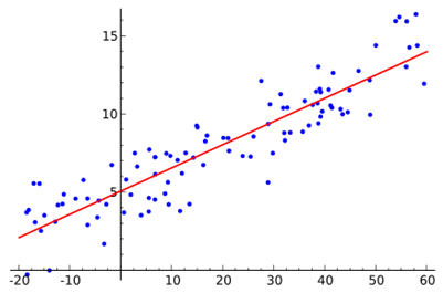
Figure 22 shows an example of simple linear regression with one independent variable (x axis). The model (red line) is calculated using training data (blue points), where each point has a known label (y axis) to fit the points as accurately as possible by minimizing the value of a chosen loss function. We can then use the model to predict unknown labels (we only know x value and want to predict y value).
Step 1. Load the dataset and create RDD
For loading the MNIST dataset in LIBSVM format, here we used the built-in API called MLUtils from Spark MLlib:
val data = MLUtils.loadLibSVMFile(spark.sparkContext, "data/mnist.bz2")
Step 2. Compute the number of features to make the dimensionality reduction easier:
val featureSize = data.first().features.size
println("Feature Size: " + featureSize)
This will result in the following output:
Feature Size: 780
So the dataset has 780 columns -i.e. features so this can be considered as high-dimensional one (features). Therefore, sometimes it is worth reducing the dimensions of the dataset.
Step 3. Now prepare the training and test set as follows:
The thing is that we will train the LinearRegressionwithSGD model twice. First, we will use the normal dataset with the original dimensions of the features, secondly, using half of the features. With the original one, the training and test set preparation go as follows:
val splits = data.randomSplit(Array(0.75, 0.25), seed = 12345L)
val (training, test) = (splits(0), splits(1))
Now, for the reduced features, the training goes as follows:
val pca = new PCA(featureSize/2).fit(data.map(_.features))
val training_pca = training.map(p => p.copy(features = pca.transform(p.features)))
val test_pca = test.map(p => p.copy(features = pca.transform(p.features)))
Step 4. Training the linear regression model
Now iterate 20 times and train the LinearRegressionWithSGD for the normal features and reduced features, respectively, as follows:
val numIterations = 20
val stepSize = 0.0001
val model = LinearRegressionWithSGD.train(training, numIterations)
val model_pca = LinearRegressionWithSGD.train(training_pca, numIterations)
Beware! Sometimes, LinearRegressionWithSGD() returns NaN. In my opinion, there are two reasons for this happening:
- If the stepSize is big. In that case, you should use something smaller, such as 0.0001, 0.001, 0.01, 0.03, 0.1, 0.3, 1.0, and so on.
- Your train data has NaN. If so, the result will likely be NaN. So, it is recommended to remove the null values prior to training the model.
Step 5. Evaluating both models
Before we evaluate the classification model, first, let's prepare for computing the MSE for the normal to see the effects of dimensionality reduction on the original predictions. Obviously, if you want a formal way to quantify the accuracy of the model and potentially increase the precision and avoid overfitting. Nevertheless, you can do from residual analysis. Also it would be worth to analyse the selection of the training and test set to be used for the model building and then the evaluation. Finally, selection techniques help you to describe the various attributes of a model:
val valuesAndPreds = test.map { point =>
                      val score = model.predict(point.features)
                      (score, point.label)
                     }
Now compute the prediction sets for the PCA one as follows:
val valuesAndPreds_pca = test_pca.map { point =>
                         val score = model_pca.predict(point.features)
                         (score, point.label)
                       }
Now compute the MSE and print them for each case as follows:
val MSE = valuesAndPreds.map { case (v, p) => math.pow(v - p 2) }.mean()
val MSE_pca = valuesAndPreds_pca.map { case (v, p) => math.pow(v - p, 2) }.mean()
println("Mean Squared Error = " + MSE)
println("PCA Mean Squared Error = " + MSE_pca)
You will get the following output:
Mean Squared Error = 2.9164359135973043E78
PCA Mean Squared Error = 2.9156682256149184E78
Note that the MSE is actually calculated using the following formula:
Step 6. Observing the model coefficient for both models
Compute the model coefficient as follows:
println("Model coefficients:"+ model.toString())
println("Model with PCA coefficients:"+ model_pca.toString())
Now you should observer the following output on your terminal/console:
Model coefficients: intercept = 0.0, numFeatures = 780
Model with PCA coefficients: intercept = 0.0, numFeatures = 390