The creation of a DataFrame can be done in several ways:
- By executing SQL queries
- Loading external data such as Parquet, JSON, CSV, text, Hive, JDBC, and so on
- Converting RDDs to data frames
A DataFrame can be created by loading a CSV file. We will look at a CSV statesPopulation.csv, which is being loaded as a DataFrame.
The CSV has the following format of US states populations from years 2010 to 2016.
| State | Year | Population |
| Alabama | 2010 | 4785492 |
| Alaska | 2010 | 714031 |
| Arizona | 2010 | 6408312 |
| Arkansas | 2010 | 2921995 |
| California | 2010 | 37332685 |
Since this CSV has a header, we can use it to quickly load into a DataFrame with an implicit schema detection.
scala> val statesDF = spark.read.option("header", "true").option("inferschema", "true").option("sep", ",").csv("statesPopulation.csv")
statesDF: org.apache.spark.sql.DataFrame = [State: string, Year: int ... 1 more field]
Once the DataFrame is loaded, it can be examined for the schema:
scala> statesDF.printSchema
root
 |-- State: string (nullable = true)
 |-- Year: integer (nullable = true)
 |-- Population: integer (nullable = true)
DataFrame works by parsing the logical plan, analyzing the logical plan, optimizing the plan, and then finally executing the physical plan of execution.
Using explain on DataFrame shows the plan of execution:
scala> statesDF.explain(true)
== Parsed Logical Plan ==
Relation[State#0,Year#1,Population#2] csv
== Analyzed Logical Plan ==
State: string, Year: int, Population: int
Relation[State#0,Year#1,Population#2] csv
== Optimized Logical Plan ==
Relation[State#0,Year#1,Population#2] csv
== Physical Plan ==
*FileScan csv [State#0,Year#1,Population#2] Batched: false, Format: CSV, Location: InMemoryFileIndex[file:/Users/salla/states.csv], PartitionFilters: [], PushedFilters: [], ReadSchema: struct<State:string,Year:int,Population:int>
A DataFrame can also be registered as a table name (shown as follows), which will then allow you to type SQL statements like a relational Database.
scala> statesDF.createOrReplaceTempView("states")
Once we have the DataFrame as a structured DataFrame or a table, we can run commands to operate on the data:
scala> statesDF.show(5)
scala> spark.sql("select * from states limit 5").show
+----------+----+----------+
| State|Year|Population|
+----------+----+----------+
| Alabama|2010| 4785492|
| Alaska|2010| 714031|
| Arizona|2010| 6408312|
| Arkansas|2010| 2921995|
|California|2010| 37332685|
+----------+----+----------+
If you see in the preceding piece of code, we have written an SQL-like statement and executed it using spark.sql API.
Note that the Spark SQL is simply converted to the DataFrame API for execution and the SQL is only a DSL for ease of use.
Using the sort operation on the DataFrame, you can order the rows in the DataFrame by any column. We see the effect of descending sort using the Population column as follows. The rows are ordered by the Population in a descending order.
scala> statesDF.sort(col("Population").desc).show(5)
scala> spark.sql("select * from states order by Population desc limit 5").show
+----------+----+----------+
| State|Year|Population|
+----------+----+----------+
|California|2016| 39250017|
|California|2015| 38993940|
|California|2014| 38680810|
|California|2013| 38335203|
|California|2012| 38011074|
+----------+----+----------+
Using groupBy we can group the DataFrame by any column. The following is the code to group the rows by State and then add up the Population counts for each State.
scala> statesDF.groupBy("State").sum("Population").show(5)
scala> spark.sql("select State, sum(Population) from states group by State limit 5").show
+---------+---------------+
| State|sum(Population)|
+---------+---------------+
| Utah| 20333580|
| Hawaii| 9810173|
|Minnesota| 37914011|
| Ohio| 81020539|
| Arkansas| 20703849|
+---------+---------------+
Using the agg operation, you can perform many different operations on columns of the DataFrame, such as finding the min, max, and avg of a column. You can also perform the operation and rename the column at the same time to suit your use case.
scala> statesDF.groupBy("State").agg(sum("Population").alias("Total")).show(5)
scala> spark.sql("select State, sum(Population) as Total from states group by State limit 5").show
+---------+--------+
| State| Total|
+---------+--------+
| Utah|20333580|
| Hawaii| 9810173|
|Minnesota|37914011|
| Ohio|81020539|
| Arkansas|20703849|
+---------+--------+
Naturally, the more complicated the logic gets, the execution plan also gets more complicated. Let's look at the plan for the preceding operation of groupBy and agg API invocations to better understand what is really going on under the hood. The following is the code showing the execution plan of the group by and summation of population per State:
scala> statesDF.groupBy("State").agg(sum("Population").alias("Total")).explain(true)

== Parsed Logical Plan ==
'Aggregate [State#0], [State#0, sum('Population) AS Total#31886]
+- Relation[State#0,Year#1,Population#2] csv

== Analyzed Logical Plan ==
State: string, Total: bigint
Aggregate [State#0], [State#0, sum(cast(Population#2 as bigint)) AS Total#31886L]
+- Relation[State#0,Year#1,Population#2] csv

== Optimized Logical Plan ==
Aggregate [State#0], [State#0, sum(cast(Population#2 as bigint)) AS Total#31886L]
+- Project [State#0, Population#2]
 +- Relation[State#0,Year#1,Population#2] csv

== Physical Plan ==
*HashAggregate(keys=[State#0], functions=[sum(cast(Population#2 as bigint))], output=[State#0, Total#31886L])
+- Exchange hashpartitioning(State#0, 200)
 +- *HashAggregate(keys=[State#0], functions=[partial_sum(cast(Population#2 as bigint))], output=[State#0, sum#31892L])
 +- *FileScan csv [State#0,Population#2] Batched: false, Format: CSV, Location: InMemoryFileIndex[file:/Users/salla/states.csv], PartitionFilters: [], PushedFilters: [], ReadSchema: struct<State:string,Population:int>
DataFrame operations can be chained together very well so that the execution takes advantage of the cost optimization (Tungsten performance improvements and catalyst optimizer working together).
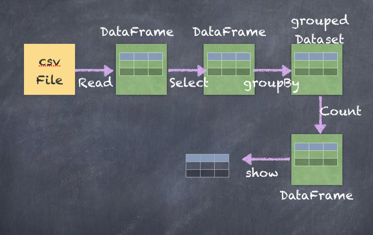
We can also chain the operations together in a single statement, as shown as follows, where we not only group the data by State column and then sum the Population value, but also sort the DataFrame by the summation column:
scala> statesDF.groupBy("State").agg(sum("Population").alias("Total")).sort(col("Total").desc).show(5)
scala> spark.sql("select State, sum(Population) as Total from states group by State order by Total desc limit 5").show
+----------+---------+
| State| Total|
+----------+---------+
|California|268280590|
| Texas|185672865|
| Florida|137618322|
| New York|137409471|
| Illinois| 89960023|
+----------+---------+
The preceding chained operation consists of multiple transformations and actions, which can be visualized using the following diagram:

It's also possible to create multiple aggregations at the same time, as follows:
scala> statesDF.groupBy("State").agg(
             min("Population").alias("minTotal"),
             max("Population").alias("maxTotal"),
             avg("Population").alias("avgTotal"))
           .sort(col("minTotal").desc).show(5)

scala> spark.sql("select State, min(Population) as minTotal, max(Population) as maxTotal, avg(Population) as avgTotal from states group by State order by minTotal desc limit 5").show
+----------+--------+--------+--------------------+
| State|minTotal|maxTotal| avgTotal|
+----------+--------+--------+--------------------+
|California|37332685|39250017|3.8325798571428575E7|
| Texas|25244310|27862596| 2.6524695E7|
| New York|19402640|19747183| 1.962992442857143E7|
| Florida|18849098|20612439|1.9659760285714287E7|
| Illinois|12801539|12879505|1.2851431857142856E7|
+----------+--------+--------+--------------------+
