In the previous section, we have seen how to load, parse, manipulate, and query the DataFrame. Now it would be great if we could show the data for better visibility. For example, what could be done for the airline carriers? I mean, is it possible to find the most frequent carriers from the plot? Let's give ggplot2 a try. At first, load the library for the same:

library(ggplot2) 

Now we already have the SparkDataFrame. What if we directly try to use our SparkSQL DataFrame class in ggplot2?

my_plot<- ggplot(data=flightDF, aes(x=factor(carrier)))
>>
ERROR: ggplot2 doesn't know how to deal with data of class SparkDataFrame.

Obviously, it doesn't work that way because the ggplot2 function doesn't know how to deal with those types of distributed data frames (the Spark ones). Instead, we need to collect the data locally and convert it back to a traditional R data frame as follows:

flight_local_df<- collect(select(flightDF,"carrier"))

Now let's have a look at what we got using the str() method as follows:

str(flight_local_df)

The output is as follows:

'data.frame':  336776 obs. of 1 variable: $ carrier: chr "UA" "UA" "AA" "B6" ...

This is good because when we collect results from a SparkSQL DataFrame, we get a regular R data.frame. It is also very convenient since we can manipulate it as needed. And now we are ready to create the ggplot2 object as follows:

my_plot<- ggplot(data=flight_local_df, aes(x=factor(carrier)))

Finally, let's give the plot a proper representation as a bar diagram as follows:

my_plot + geom_bar() + xlab("Carrier")

The output is as follows:

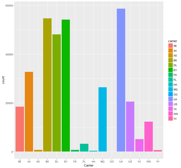
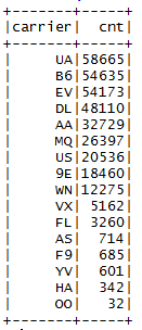
From the graph, it is clear that the most frequent carriers are UA, B6, EV, and DL. This gets clearer from the following line of code in R:

carrierDF = sql("SELECT carrier, COUNT(*) as cnt FROM flight GROUP BY carrier ORDER BY cnt DESC")
showDF(carrierDF)

The output is as follows:

The full source code of the preceding analysis is given in the following to understand the flow of the code:

#Configure SparkR
SPARK_HOME = "C:/Users/rezkar/Downloads/spark-2.1.0-bin-hadoop2.7/R/lib"
HADOOP_HOME= "C:/Users/rezkar/Downloads/spark-2.1.0-bin-hadoop2.7/bin"
Sys.setenv(SPARK_MEM = "2g")
Sys.setenv(SPARK_HOME = "C:/Users/rezkar/Downloads/spark-2.1.0-bin-hadoop2.7")
.libPaths(c(file.path(Sys.getenv("SPARK_HOME"), "R", "lib"), .libPaths()))

#Load SparkR
library(SparkR, lib.loc = SPARK_HOME)

# Initialize SparkSession
sparkR.session(appName = "Example", master = "local[*]", sparkConfig = list(spark.driver.memory = "8g"))
# Point the data file path:
dataPath<- "C:/Exp/nycflights13.csv"

#Creating DataFrame using external data source API
flightDF<- read.df(dataPath,
header='true',
source = "com.databricks.spark.csv",
inferSchema='true')
printSchema(flightDF)
showDF(flightDF, numRows = 10)
# Using SQL to select columns of data

# First, register the flights SparkDataFrame as a table
createOrReplaceTempView(flightDF, "flight")
destDF<- sql("SELECT dest, origin, carrier FROM flight")
showDF(destDF, numRows=10)

#And then we can use SparkR sql function using condition as follows:
selected_flight_SQL<- sql("SELECT dest, origin, arr_delay FROM flight WHERE arr_delay>= 120")
showDF(selected_flight_SQL, numRows = 10)

#Bit complex query: Let's find the origins of all the flights that are at least 2 hours delayed where the destiantionn is Iowa. Finally, sort them by arrival delay and limit the count upto 20 and the destinations
selected_flight_SQL_complex<- sql("SELECT origin, dest, arr_delay FROM flight WHERE dest='IAH' AND arr_delay>= 120 ORDER BY arr_delay DESC LIMIT 20")
showDF(selected_flight_SQL_complex)

# Stop the SparkSession now
sparkR.session.stop()