Now we will show you how to predict the possibility of breast cancer with step-by-step example:

Step 1: Load and parse the data

val rdd = spark.sparkContext.textFile("data/wbcd.csv") 
val cancerRDD = parseRDD(rdd).map(parseCancer) 

The parseRDD() method goes as follows:

def parseRDD(rdd: RDD[String]): RDD[Array[Double]] = { 
  rdd.map(_.split(",")).filter(_(6) != "?").map(_.drop(1)).map(_.map(_.toDouble)) 
} 

The parseCancer() method is as follows:

def parseCancer(line: Array[Double]): Cancer = { 
  Cancer(if (line(9) == 4.0) 1 else 0, line(0), line(1), line(2), line(3), line(4), line(5), line(6), line(7), line(8)) 
}  

Note that here we have simplified the dataset. For the value 4.0, we have converted them to 1.0, and 0.0 otherwise. The Cancer class is a case class that can be defined as follows:

case class Cancer(cancer_class: Double, thickness: Double, size: Double, shape: Double, madh: Double, epsize: Double, bnuc: Double, bchrom: Double, nNuc: Double, mit: Double)

Step 2: Convert RDD to DataFrame for the ML pipeline

import spark.sqlContext.implicits._
val cancerDF = cancerRDD.toDF().cache() 
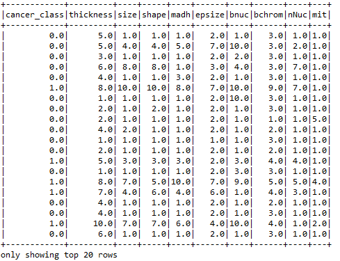
cancerDF.show() 

The DataFrame looks like the following:

Step 3: Feature extraction and transformation

At first, let's select the feature column, as follows:

val featureCols = Array("thickness", "size", "shape", "madh", "epsize", "bnuc", "bchrom", "nNuc", "mit") 

Now let's assemble them into a feature vector, as follows:

val assembler = new VectorAssembler().setInputCols(featureCols).setOutputCol("features") 

Now transform them into a DataFrame, as follows:

val df2 = assembler.transform(cancerDF) 

Let's see the structure of the transformed DataFrame:

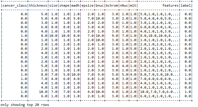
df2.show() 

Now you should observe a DataFrame containing the features calculated based on the columns on the left:

Finally, let's use the StringIndexer and create the label for the training dataset, as follows:

val labelIndexer = new StringIndexer().setInputCol("cancer_class").setOutputCol("label")
val df3 = labelIndexer.fit(df2).transform(df2)
df3.show() 

Now you should observe a DataFrame containing the features and labels calculated based on the columns in the left:

Step 4: Create test and training set

val splitSeed = 1234567 
val Array(trainingData, testData) = df3.randomSplit(Array(0.7, 0.3), splitSeed)

Step 5: Creating an estimator using the training sets

Let's create an estimator for the pipeline using the logistic regression with elasticNetParam. We also specify the max iteration and regression parameter, as follows:

val lr = new LogisticRegression().setMaxIter(50).setRegParam(0.01).setElasticNetParam(0.01) 
val model = lr.fit(trainingData)  

Step 6: Getting raw prediction, probability, and prediction for the test set

Transform the model using the test set to get raw prediction, probability, and prediction for the test set:

val predictions = model.transform(testData) 
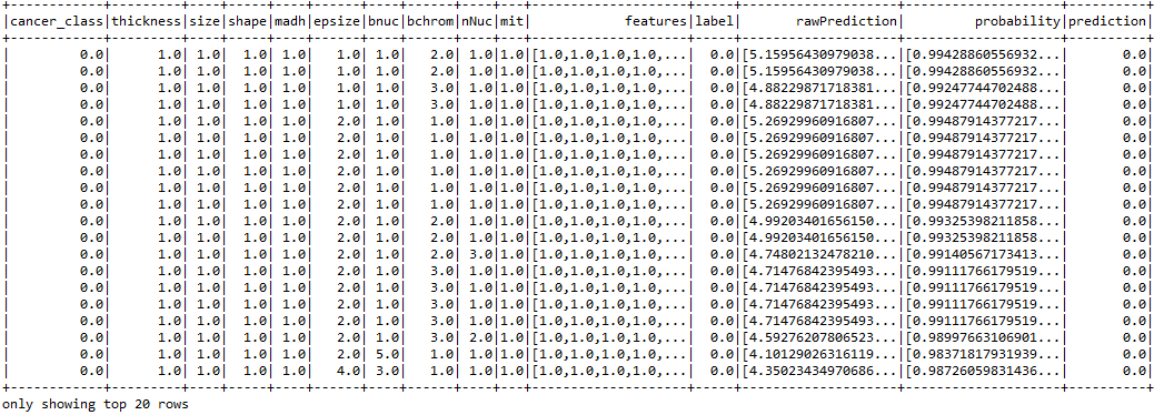
predictions.show() 

The resulting DataFrame is as follows:

Step 7: Generating objective history of training

Let's generate the objective history of the model in each iteration, as follows:

val trainingSummary = model.summary 
val objectiveHistory = trainingSummary.objectiveHistory 
objectiveHistory.foreach(loss => println(loss))

The preceding code segment produces the following output in terms of training loss:

    0.6562291876496595
    0.6087867761081431
    0.538972588904556
    0.4928455913405332
    0.46269258074999386
    0.3527914819973198
    0.20206901337404978
    0.16459454874996993
    0.13783437051276512
    0.11478053164710095
    0.11420433621438157
    0.11138884788059378
    0.11041889032338036
    0.10849477236373875
    0.10818880537879513
    0.10682868640074723
    0.10641395229253267
    0.10555411704574749
    0.10505186414044905
    0.10470425580130915
    0.10376219754747162
    0.10331139609033112
    0.10276173290225406
    0.10245982201904923
    0.10198833366394071
    0.10168248313103552
    0.10163242551955443
    0.10162826209311404
    0.10162119367292953
    0.10161235376791203
    0.1016114803209495
    0.10161090505556039
    0.1016107261254795
    0.10161056082112738
    0.10161050381332608
    0.10161048515341387
    0.10161043900301985
    0.10161042057436288
    0.10161040971267737
    0.10161040846923354
    0.10161040625542347
    0.10161040595207525
    0.10161040575664354
    0.10161040565870835
    0.10161040519559975
    0.10161040489834573
    0.10161040445215266
    0.1016104043469577
    0.1016104042793553
    0.1016104042606048
    0.10161040423579716 

As you can see, the loss gradually reduces in later iterations.

Step 8: Evaluating the model

First, we will have to make sure that the classifier that we used comes from the binary logistic regression summary:

val binarySummary = trainingSummary.asInstanceOf[BinaryLogisticRegressionSummary]

Now let's obtain the ROC as a DataFrame and areaUnderROC. A value approximate to 1.0 is better:

val roc = binarySummary.roc 
roc.show() 
println("Area Under ROC: " + binarySummary.areaUnderROC)

The preceding lines prints the value of areaUnderROC, as follows:

Area Under ROC: 0.9959095884623509

This is excellent! Now let's compute other metrics, such as true positive rate, false positive rate, false negative rate, and total count, and a number of instances correctly and wrongly predicted, as follows:

import org.apache.spark.sql.functions._

// Calculate the performance metrics
val lp = predictions.select("label", "prediction") 
val counttotal = predictions.count() 
val correct = lp.filter($"label" === $"prediction").count() 
val wrong = lp.filter(not($"label" === $"prediction")).count() 
val truep = lp.filter($"prediction" === 0.0).filter($"label" === $"prediction").count() 
val falseN = lp.filter($"prediction" === 0.0).filter(not($"label" === $"prediction")).count() 
val falseP = lp.filter($"prediction" === 1.0).filter(not($"label" === $"prediction")).count() 
val ratioWrong = wrong.toDouble / counttotal.toDouble 
val ratioCorrect = correct.toDouble / counttotal.toDouble 
 
println("Total Count: " + counttotal) 
println("Correctly Predicted: " + correct) 
println("Wrongly Identified: " + wrong) 
println("True Positive: " + truep) 
println("False Negative: " + falseN) 
println("False Positive: " + falseP) 
println("ratioWrong: " + ratioWrong) 
println("ratioCorrect: " + ratioCorrect) 

Now you should observe an output from the preceding code as follows:

Total Count: 209
Correctly Predicted: 202
Wrongly Identified: 7
True Positive: 140
False Negative: 4
False Positive: 3
ratioWrong: 0.03349282296650718
ratioCorrect: 0.9665071770334929

Finally, let's judge the accuracy of the model. However, first, we need to set the model threshold to maximize fMeasure:

val fMeasure = binarySummary.fMeasureByThreshold 
val fm = fMeasure.col("F-Measure") 
val maxFMeasure = fMeasure.select(max("F-Measure")).head().getDouble(0) 
val bestThreshold = fMeasure.where($"F-Measure" === maxFMeasure).select("threshold").head().getDouble(0) 
model.setThreshold(bestThreshold) 

Now let's compute the accuracy, as follows:

val evaluator = new BinaryClassificationEvaluator().setLabelCol("label") 
val accuracy = evaluator.evaluate(predictions) 
println("Accuracy: " + accuracy)     

The preceding code produces the following output, which is almost 99.64%:

Accuracy: 0.9963975418520874