Anomalous data refers to data that is unusual from normal distributions. Thus, detecting anomalies is an important task for network security, anomalous packets or requests can be flagged as errors or potential attacks.
In this example, we will use the KDD-99 dataset (can be downloaded here: http://kdd.ics.uci.edu/databases/kddcup99/kddcup99.html ). A number of columns will be filtered out based on certain criteria of the data points. This will help us understand the example. Secondly, for the unsupervised task; we will have to remove the labeled data. Let's load and parse the dataset as simple texts. Then let's see how many rows there are in the dataset:
INPUT = "C:/Users/rezkar/Downloads/kddcup.data"
spark = SparkSession
         .builder
         .appName("PCAExample")
         .getOrCreate()

 kddcup_data = spark.sparkContext.textFile(INPUT)
This essentially returns an RDD. Let's see how many rows in the dataset are using the count() method as follows:
count = kddcup_data.count()
print(count)>>4898431
So, the dataset is pretty big with lots of features. Since we have parsed the dataset as simple texts, we should not expect to see the better structure of the dataset. Thus, let's work toward converting the RDD into DataFrame as follows:
kdd = kddcup_data.map(lambda l: l.split(","))
from pyspark.sql import SQLContext
sqlContext = SQLContext(spark)
df = sqlContext.createDataFrame(kdd)
Then let's see some selected columns in the DataFrame as follows:
df.select("_1", "_2", "_3", "_4", "_42").show(5)
The output is as follows:
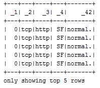
Thus, this dataset is already labeled. This means that the types of malicious cyber behavior have been assigned to a row where the label is the last column (that is, _42). The first five rows off the DataFrame are labeled normal. This means that these data points are normal. Now this is the time that we need to determine the counts of the labels for the entire dataset for each type of labels:
#Identifying the labels for unsupervised task
labels = kddcup_data.map(lambda line: line.strip().split(",")[-1])
from time import time
start_label_count = time()
label_counts = labels.countByValue()
label_count_time = time()-start_label_count

from collections import OrderedDict
sorted_labels = OrderedDict(sorted(label_counts.items(), key=lambda t: t[1], reverse=True))
for label, count in sorted_labels.items():
       print label, count
The output is as follows:

We can see that there are 23 distinct labels (behavior for data objects). The most data points belong to Smurf. This is an abnormal behavior also known as DoS packet floods. The Neptune is the second highest abnormal behavior. The normal events are the third most occurring types of events in the dataset. However, in a real network dataset, you will not see any such labels.
Also, the normal traffic will be much higher than any anomalous traffic. As a result, identifying the anomalous attack or anomaly from the large-scale unlabeled data would be tedious. For simplicity, let's ignore the last column (that is, labels) and think that this dataset is unlabeled too. In that case, the only way to conceptualize the anomaly detection is using unsupervised learning algorithms such as k-means for clustering.
Now let's work toward clustering the data points for this. One important thing about K-means is that it only accepts numeric values for modeling. However, our dataset also contains some categorical features. Now we can assign the categorical features binary values of 1 or 0 based on whether they are TCP or not. This can be done as follows:
from numpy import array
def parse_interaction(line):
     line_split = line.split(",")
     clean_line_split = [line_split[0]]+line_split[4:-1]
     return (line_split[-1], array([float(x) for x in clean_line_split]))

 parsed_data = kddcup_data.map(parse_interaction)
 pd_values = parsed_data.values().cache()
Thus, our dataset is almost ready. Now we can prepare our training and test set to training the k-means model with ease:
 kdd_train = pd_values.sample(False, .75, 12345)
 kdd_test = pd_values.sample(False, .25, 12345)
 print("Training set feature count: " + str(kdd_train.count()))
 print("Test set feature count: " + str(kdd_test.count()))
The output is as follows:
Training set feature count: 3674823
Test set feature count: 1225499
However, some standardization is also required since we converted some categorical features to numeric features. Standardization can improve the convergence rate during the optimization process and can also prevent features with very large variances exerting an influence during model training.
Now we will use StandardScaler, which is a feature transformer. It helps us standardize features by scaling them to unit variance. It then sets the mean to zero using column summary statistics in the training set samples:
standardizer = StandardScaler(True, True)
Now let's compute the summary statistics by fitting the preceding transformer as follows:
standardizer_model = standardizer.fit(kdd_train)
Now the problem is the data that we have for training the k-means does not have a normal distribution. Thus, we need to normalize each feature in the training set to have the unit standard deviation. To make this happen, we need to further transform the preceding standardizer model as follows:
data_for_cluster = standardizer_model.transform(kdd_train)
Well done! Now the training set is finally ready to train the k-means model. As we discussed in the clustering chapter, the trickiest thing in the clustering algorithm is finding the optimal number of clusters by setting the value of K so that the data objects get clustered automatically.
One Naive approach considered a brute force is setting K=2 and observing the results and trying until you get an optimal one. However, a much better approach is the Elbow approach, where we can keep increasing the value of K and compute the Within Set Sum of Squared Errors (WSSSE) as the clustering cost. In short, we will be looking for the optimal K values that also minimize the WSSSE. Whenever a sharp decrease is observed, we will get to know the optimal value for K:
import numpy
our_k = numpy.arange(10, 31, 10)
metrics = []
def computeError(point):
 center = clusters.centers[clusters.predict(point)]
 denseCenter = DenseVector(numpy.ndarray.tolist(center))
return sqrt(sum([x**2 for x in (DenseVector(point.toArray()) - denseCenter)]))
for k in our_k:
      clusters = KMeans.train(data_for_cluster, k, maxIterations=4, initializationMode="random")
      WSSSE = data_for_cluster.map(lambda point: computeError(point)).reduce(lambda x, y: x + y)
      results = (k, WSSSE)
 metrics.append(results)
print(metrics)
The output is as follows:
[(10, 3364364.5203123973), (20, 3047748.5040717563), (30, 2503185.5418753517)]
In this case, 30 is the best value for k. Let's check the cluster assignments for each data point when we have 30 clusters. The next test would be to run for k values of 30, 35, and 40. Three values of k are not the most you would test in a single run, but only used for this example:
modelk30 = KMeans.train(data_for_cluster, 30, maxIterations=4, initializationMode="random")
 cluster_membership = data_for_cluster.map(lambda x: modelk30.predict(x))
 cluster_idx = cluster_membership.zipWithIndex()
 cluster_idx.take(20)
 print("Final centers: " + str(modelk30.clusterCenters))
The output is as follows:

Now let's compute and print the total cost for the overall clustering as follows:
print("Total Cost: " + str(modelk30.computeCost(data_for_cluster)))
The output is as follows:
Total Cost: 68313502.459
Finally, the WSSSE of our k-means model can be computed and printed as follows:
WSSSE = data_for_cluster.map(lambda point: computeError
(point)).reduce(lambda x, y: x + y)
 print("WSSSE: " + str(WSSSE))
The output is as follows:
WSSSE: 2503185.54188
Your results might be slightly different. This is due to the random placement of the centroids when we first begin the clustering algorithm. Performing this many times allows you to see how points in your data change their value of k or stay the same. The full source code for this solution is given in the following:
import os
import sys
import numpy as np
from collections import OrderedDict

try:
    from collections import OrderedDict
    from numpy import array
    from math import sqrt
    import numpy
    import urllib
    import pyspark
    from pyspark.sql import SparkSession
    from pyspark.mllib.feature import StandardScaler
    from pyspark.mllib.clustering import KMeans, KMeansModel
    from pyspark.mllib.linalg import DenseVector
    from pyspark.mllib.linalg import SparseVector
    from collections import OrderedDict
    from time import time
    from pyspark.sql.types import *
    from pyspark.sql import DataFrame
    from pyspark.sql import SQLContext
    from pyspark.sql import Row
    print("Successfully imported Spark Modules")

except ImportError as e:
    print ("Can not import Spark Modules", e)
    sys.exit(1)

spark = SparkSession
        .builder
        .appName("PCAExample")
        .getOrCreate()

INPUT = "C:/Exp/kddcup.data.corrected"
kddcup_data = spark.sparkContext.textFile(INPUT)
count = kddcup_data.count()
print(count)
kddcup_data.take(5)
kdd = kddcup_data.map(lambda l: l.split(","))
sqlContext = SQLContext(spark)
df = sqlContext.createDataFrame(kdd)
df.select("_1", "_2", "_3", "_4", "_42").show(5)

#Identifying the leabels for unsupervised task
labels = kddcup_data.map(lambda line: line.strip().split(",")[-1])
start_label_count = time()
label_counts = labels.countByValue()
label_count_time = time()-start_label_count

sorted_labels = OrderedDict(sorted(label_counts.items(), key=lambda t: t[1], reverse=True))
for label, count in sorted_labels.items():
    print(label, count)

def parse_interaction(line):
    line_split = line.split(",")
    clean_line_split = [line_split[0]]+line_split[4:-1]
    return (line_split[-1], array([float(x) for x in clean_line_split]))

parsed_data = kddcup_data.map(parse_interaction)
pd_values = parsed_data.values().cache()

kdd_train = pd_values.sample(False, .75, 12345)
kdd_test = pd_values.sample(False, .25, 12345)
print("Training set feature count: " + str(kdd_train.count()))
print("Test set feature count: " + str(kdd_test.count()))

standardizer = StandardScaler(True, True)
standardizer_model = standardizer.fit(kdd_train)
data_for_cluster = standardizer_model.transform(kdd_train)

initializationMode="random"

our_k = numpy.arange(10, 31, 10)
metrics = []

def computeError(point):
    center = clusters.centers[clusters.predict(point)]
    denseCenter = DenseVector(numpy.ndarray.tolist(center))
    return sqrt(sum([x**2 for x in (DenseVector(point.toArray()) - denseCenter)]))

for k in our_k:
     clusters = KMeans.train(data_for_cluster, k, maxIterations=4, initializationMode="random")
     WSSSE = data_for_cluster.map(lambda point: computeError(point)).reduce(lambda x, y: x + y)
     results = (k, WSSSE)
     metrics.append(results)
print(metrics)

modelk30 = KMeans.train(data_for_cluster, 30, maxIterations=4, initializationMode="random")
cluster_membership = data_for_cluster.map(lambda x: modelk30.predict(x))
cluster_idx = cluster_membership.zipWithIndex()
cluster_idx.take(20)
print("Final centers: " + str(modelk30.clusterCenters))
print("Total Cost: " + str(modelk30.computeCost(data_for_cluster)))
WSSSE = data_for_cluster.map(lambda point: computeError(point)).reduce(lambda x, y: x + y)
print("WSSSE" + str(WSSSE))
Well, now it's time to move to SparkR, another Spark API to work with population statistical programming language called R.