A binary logistic regression can be generalized into multinomial logistic regression to train and predict multiclass classification problems. For example, for K possible outcomes, one of the outcomes can be chosen as a pivot, and the other K−1 outcomes can be separately regressed against the pivot outcome. In spark.mllib, the first class 0 is chosen as the pivot class.

For multiclass classification problems, the algorithm will output a multinomial logistic regression model, which contains k−1binary logistic regression models regressed against the first class. Given a new data point, k−1models will be run, and the class with the largest probability will be chosen as the predicted class. In this section, we will show you an example of a classification using the logistic regression with L-BFGS for faster convergence.

Step 1. Load and parse the MNIST dataset in LIVSVM format

// Load training data in LIBSVM format.
 val data = MLUtils.loadLibSVMFile(spark.sparkContext, "data/mnist.bz2")

Step 2. Prepare the training and test sets

Split data into training (75%) and test (25%), as follows:

val splits = data.randomSplit(Array(0.75, 0.25), seed = 12345L)
val training = splits(0).cache()
val test = splits(1)

Step 3. Run the training algorithm to build the model

Run the training algorithm to build the model by setting a number of classes (10 for this dataset). For better classification accuracy, you can also specify intercept and validate the dataset using the Boolean true value, as follows:

val model = new LogisticRegressionWithLBFGS()
           .setNumClasses(10)
           .setIntercept(true)
           .setValidateData(true)
           .run(training)

Set intercept as true if the algorithm should add an intercept using setIntercept(). If you want the algorithm to validate the training set before the model building itself, you should set the value as true using the setValidateData() method.

Step 4. Clear the default threshold

Clear the default threshold so that the training does not occur with the default setting, as follows:

model.clearThreshold()

Step 5. Compute raw scores on the test set

Compute raw scores on the test set so that we can evaluate the model using the aforementioned performance metrics, as follows:

val scoreAndLabels = test.map { point =>
  val score = model.predict(point.features)
  (score, point.label)
}

Step 6. Instantiate a multiclass metrics for the evaluation

val metrics = new MulticlassMetrics(scoreAndLabels)

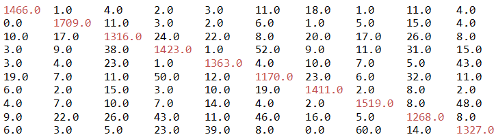
Step 7. Constructing the confusion matrix

println("Confusion matrix:")
println(metrics.confusionMatrix)

In a confusion matrix, each column of the matrix represents the instances in a predicted class, while each row represents the instances in an actual class (or vice versa). The name stems from the fact that it makes it easy to see if the system is confusing two classes. For more, refer to matrix (https://en.wikipedia.org/wiki/Confusion_matrix.Confusion):

Step 8. Overall statistics

Now let's compute the overall statistics to judge the performance of the model:

val accuracy = metrics.accuracy
println("Summary Statistics")
println(s"Accuracy = $accuracy")
// Precision by label
val labels = metrics.labels
labels.foreach { l =>
  println(s"Precision($l) = " + metrics.precision(l))
}
// Recall by label
labels.foreach { l =>
  println(s"Recall($l) = " + metrics.recall(l))
}
// False positive rate by label
labels.foreach { l =>
  println(s"FPR($l) = " + metrics.falsePositiveRate(l))
}
// F-measure by label
labels.foreach { l =>
  println(s"F1-Score($l) = " + metrics.fMeasure(l))
}

The preceding code segment produces the following output, containing some performance metrics, such as accuracy, precision, recall, true positive rate , false positive rate, and f1 score:

Summary Statistics
 ----------------------
 Accuracy = 0.9203609775377116
 Precision(0.0) = 0.9606815203145478
 Precision(1.0) = 0.9595732734418866
 .
 .
 Precision(8.0) = 0.8942172073342737
 Precision(9.0) = 0.9027210884353741
 
 Recall(0.0) = 0.9638395792241946
 Recall(1.0) = 0.9732346241457859
 .
 .
 Recall(8.0) = 0.8720770288858322
 Recall(9.0) = 0.8936026936026936
 
 FPR(0.0) = 0.004392386530014641
 FPR(1.0) = 0.005363128491620112
 .
 .
 FPR(8.0) = 0.010927369417935456
 FPR(9.0) = 0.010441004672897197
 
 F1-Score(0.0) = 0.9622579586478502
 F1-Score(1.0) = 0.966355668645745
 .
 .
 F1-Score(9.0) = 0.8981387478849409

Now let's compute the overall, that is, summary statistics:

println(s"Weighted precision: ${metrics.weightedPrecision}")
println(s"Weighted recall: ${metrics.weightedRecall}")
println(s"Weighted F1 score: ${metrics.weightedFMeasure}")
println(s"Weighted false positive rate: ${metrics.weightedFalsePositiveRate}") 

The preceding code segment prints the following output containing weighted precision, recall, f1 score, and false positive rate:

Weighted precision: 0.920104303076327
 Weighted recall: 0.9203609775377117
 Weighted F1 score: 0.9201934861645358
 Weighted false positive rate: 0.008752250453215607

The overall statistics say that the accuracy of the model is more than 92%. However, we can still improve it using a better algorithm such as random forest (RF). In the next section, we will look at the random forest implementation to classify the same model.