As you have already seen, using the OVTR classifier we observed the following values of the performance metrics on the OCR dataset:
Accuracy = 0.5217246545696688
Precision = 0.488360500637862
Recall = 0.5217246545696688
F1 = 0.4695649096879411
Test Error = 0.47827534543033123
This signifies that the accuracy of the model on that dataset is very low. In this section, we will see how we could improve the performance using the DT classifier. An example with Spark 2.1.0 will be shown using the same OCR dataset. The example will have several steps including data loading, parsing, model training, and, finally, model evaluation.
Since we will be using the same dataset, to avoid redundancy, we will escape the dataset exploration step and will enter into the example:
Step 1. Load the required library and packages as follows:
import org.apache.spark.ml.Pipeline // for Pipeline creation
import org.apache.spark.ml.classification
                         .DecisionTreeClassificationModel
import org.apache.spark.ml.classification.DecisionTreeClassifier
import org.apache.spark.ml.evaluation
                         .MulticlassClassificationEvaluator
import org.apache.spark.ml.feature
                         .{IndexToString, StringIndexer, VectorIndexer}
import org.apache.spark.sql.SparkSession //For a Spark session
Step 2. Create an active Spark session as follows:
val spark = SparkSession
              .builder
              .master("local[*]")
              .config("spark.sql.warehouse.dir", "/home/exp/")
              .appName("DecisionTreeClassifier")
              .getOrCreate()
Note that here the master URL has been set as local[*], which means all the cores of your machine will be used for processing the Spark job. You should set SQL warehouse accordingly and other configuration parameter based on requirements.
Step 3. Create the DataFrame - Load the data stored in LIBSVM format as a DataFrame as follows:
val data = spark.read.format("libsvm").load("datab
                             /Letterdata_libsvm.data")
For the classification of digits, the input feature vectors are usually sparse, and sparse vectors should be supplied as input to take advantage of the sparsity. Since the training data is only used once, and moreover the size of the dataset is relatively small (that is, a few MBs), we can cache it if you use the DataFrame more than once.
Step 4. Label indexing - Index the labels, adding metadata to the label column. Then let's fit on the whole dataset to include all labels in the index:
val labelIndexer = new StringIndexer()
               .setInputCol("label")
               .setOutputCol("indexedLabel")
               .fit(data)
Step 5. Identifying categorical features - The following code segment automatically identifies categorical features and indexes them:
val featureIndexer = new VectorIndexer()
              .setInputCol("features")
              .setOutputCol("indexedFeatures")
              .setMaxCategories(4)
              .fit(data)
For this case, if the number of features is more than four distinct values, they will be treated as continuous.
Step 6. Prepare the training and test sets - Split the data into training and test sets (25% held out for testing):
val Array(trainingData, testData) = data.randomSplit
                                      (Array(0.75, 0.25), 12345L)
Step 7. Train the DT model as follows:
val dt = new DecisionTreeClassifier()
                     .setLabelCol("indexedLabel")
                     .setFeaturesCol("indexedFeatures")
Step 8. Convert the indexed labels back to original labels as follows:
val labelConverter = new IndexToString()
                .setInputCol("prediction")
                .setOutputCol("predictedLabel")
                .setLabels(labelIndexer.labels)
Step 9. Create a DT pipeline - Let's create a DT pipeline by changing the indexers, label converter and tree together:
val pipeline = new Pipeline().setStages(Array(labelIndexer,
                              featureIndexer, dt, labelconverter))
Step 10. Running the indexers - Train the model using the transformer and run the indexers:
val model = pipeline.fit(trainingData)
Step 11. Calculate the prediction on the test set - Calculate the prediction using the model transformer and finally show the prediction against each label as follows:
val predictions = model.transform(testData)
predictions.show()
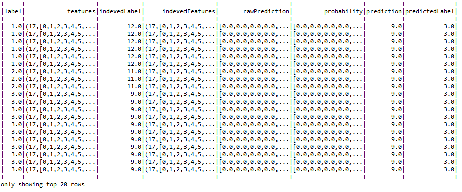
As you can see from the preceding figure, some labels were predicted accurately and some of them were predicted wrongly. However, we know the weighted accuracy, precision, recall, and f1 measures, but we need to evaluate the model first.
Step 12. Evaluate the model - Select the prediction and the true label to compute test error and classification performance metrics such as accuracy, precision, recall, and f1 measure as follows:
val evaluator = new MulticlassClassificationEvaluator()
                             .setLabelCol("label")
                             .setPredictionCol("prediction")
val evaluator1 = evaluator.setMetricName("accuracy")
val evaluator2 = evaluator.setMetricName("weightedPrecision")
val evaluator3 = evaluator.setMetricName("weightedRecall")
val evaluator4 = evaluator.setMetricName("f1")
Step 13. Compute the performance metrics - Compute the classification accuracy, precision, recall, f1 measure, and error on test data as follows:
val accuracy = evaluator1.evaluate(predictions)
val precision = evaluator2.evaluate(predictions)
val recall = evaluator3.evaluate(predictions)
val f1 = evaluator4.evaluate(predictions)
Step 14. Print the performance metrics:
println("Accuracy = " + accuracy)
println("Precision = " + precision)
println("Recall = " + recall)
println("F1 = " + f1)
println(s"Test Error = ${1 - accuracy}")
You should observe values as follows:
Accuracy = 0.994277821625888
Precision = 0.9904583933020722
Recall = 0.994277821625888
F1 = 0.9919966504321712
Test Error = 0.005722178374112041
Now the performance is excellent, right? However, you can still increase the classification accuracy by performing hyperparameter tuning. There are further opportunities to improve the prediction accuracy by selecting appropriate algorithms (that is, classifier or regressor) through cross-validation and train split.
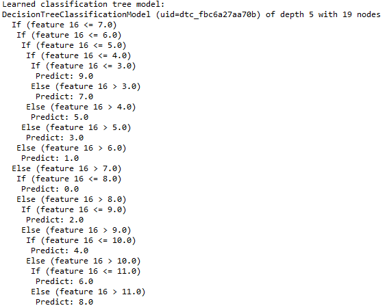
Step 15. Print the DT nodes:
val treeModel = model.stages(2).asInstanceOf
                                [DecisionTreeClassificationModel]
println("Learned classification tree model:
" + treeModel
                 .toDebugString)
Finally, we will print a few nodes in the DT, as shown in the following figure: