
PCA is good at reducing the number of dimensions, but it works in a linear manner. If the data is not organized in a linear fashion, PCA fails to do the required job. This is where Kernel PCA comes into the picture. You can learn more about it at http://www.ics.uci.edu/~welling/classnotes/papers_class/Kernel-PCA.pdf. Let's see how to perform Kernel PCA on the input data and compare it to how PCA performs on the same data.
- Create a new Python file, and import the following packages:
import numpy as np
import matplotlib.pyplot as plt

from sklearn.decomposition import PCA, KernelPCA
from sklearn.datasets import make_circles
- Define the seed value for the random number generator. This is needed to generate the data samples for analysis:
# Set the seed for random number generator
np.random.seed(7)
- Generate data that is distributed in concentric circles to demonstrate how PCA doesn't work in this case:
# Generate samples
X, y = make_circles(n_samples=500, factor=0.2, noise=0.04)
- Perform PCA on this data:
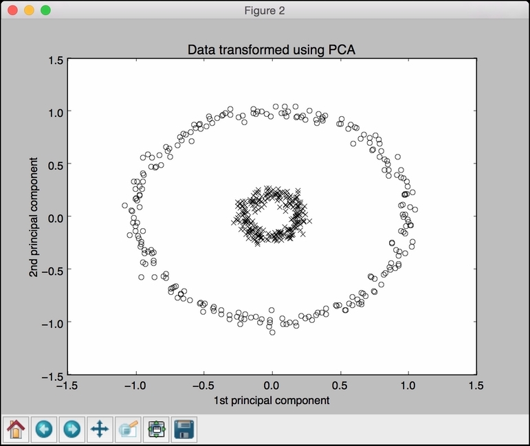
# Perform PCA
pca = PCA()
X_pca = pca.fit_transform(X)
- Perform Kernel PCA on this data:
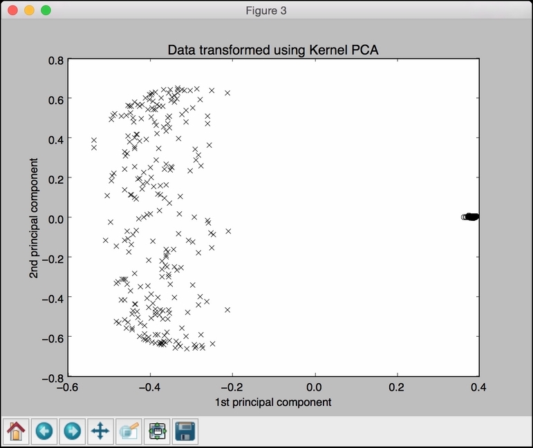
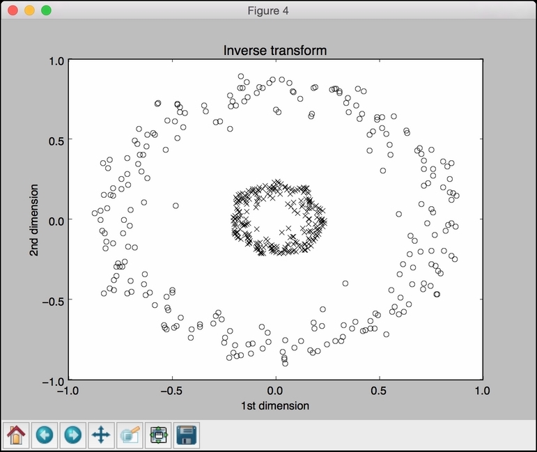
# Perform Kernel PCA
kernel_pca = KernelPCA(kernel="rbf", fit_inverse_transform=True, gamma=10)
X_kernel_pca = kernel_pca.fit_transform(X)
X_inverse = kernel_pca.inverse_transform(X_kernel_pca)
- Plot the original input data:
# Plot original data class_0 = np.where(y == 0) class_1 = np.where(y == 1) plt.figure() plt.title("Original data") plt.plot(X[class_0, 0], X[class_0, 1], "ko", mfc='none') plt.plot(X[class_1, 0], X[class_1, 1], "kx") plt.xlabel("1st dimension") plt.ylabel("2nd dimension") - Plot the PCA-transformed data:
# Plot PCA projection of the data plt.figure() plt.plot(X_pca[class_0, 0], X_pca[class_0, 1], "ko", mfc='none') plt.plot(X_pca[class_1, 0], X_pca[class_1, 1], "kx") plt.title("Data transformed using PCA") plt.xlabel("1st principal component") plt.ylabel("2nd principal component") - Plot Kernel PCA-transformed data:
# Plot Kernel PCA projection of the data plt.figure() plt.plot(X_kernel_pca[class_0, 0], X_kernel_pca[class_0, 1], "ko", mfc='none') plt.plot(X_kernel_pca[class_1, 0], X_kernel_pca[class_1, 1], "kx") plt.title("Data transformed using Kernel PCA") plt.xlabel("1st principal component") plt.ylabel("2nd principal component") - Transform the data back to the original space using the Kernel method to show that the inverse is maintained:
# Transform the data back to original space plt.figure() plt.plot(X_inverse[class_0, 0], X_inverse[class_0, 1], "ko", mfc='none') plt.plot(X_inverse[class_1, 0], X_inverse[class_1, 1], "kx") plt.title("Inverse transform") plt.xlabel("1st dimension") plt.ylabel("2nd dimension") plt.show() - The full code is given in the
kpca.pyfile that's already provided to you for reference. If you run this code, you will see four figures. The first figure is the original data: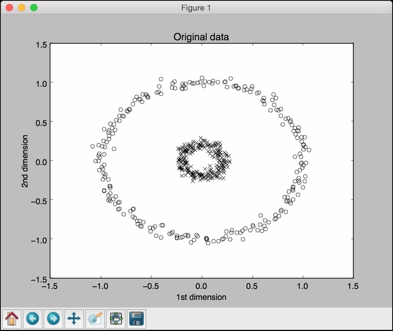
The second figure depicts the data transformed using PCA:
The third figure depicts the data transformed using Kernel PCA. Note how the points are clustered in the right part of the figure:
The fourth figure depicts the inverse transform of the data back to the original space:
..................Content has been hidden....................
You can't read the all page of ebook, please click here login for view all page.