A Boltzmann machine is a particular type of stochastic, recurrent neural network. It is an energy-based model, which means that it uses an energy function to associate an energy value with each configuration of the network.

We briefly discussed the structure of a Boltzmann machine in the previous section. As mentioned, a Boltzmann machine is a directed cyclic graph, where every node is connected to all other nodes. This property enables it to model in a recurrent fashion, such that the model's outputs evolve and can be viewed over time.

The learning loop in a Boltzmann machine involves maximizing the probability of the training dataset, X. As noted, the specific performance measure used is energy, which is characterized as the negative log of the probability for a dataset X, given a vector of model parameters, Θ. This measure is calculated and used to update the network's weights in such a way as to minimize the free energy in the network.

The Boltzmann machine has seen particular success in processing image data, including photographs, facial features, and handwriting classification contexts.

Unfortunately, the Boltzmann machine is not practical for more challenging ML problems. This is due to the fact that there are challenges with the machine's ability to scale; as the number of nodes increases, the compute time grows exponentially, eventually leaving us in a position where we're unable to compute the free energy of the network.

In order to overcome the weaknesses of the Boltzmann machine, it is necessary to make adjustments to both the network topology and training process.

Topology

The main topological change that delivers efficiency improvements is the restriction of connectivity between nodes. First, one must prevent connection between nodes within the same layer. Additionally, all skip-layer connections (that is, direct connections between non-consecutive layers) must be prevented. A Boltzmann machine with this architecture is referred to as an RBM and appears as shown in the following diagram:

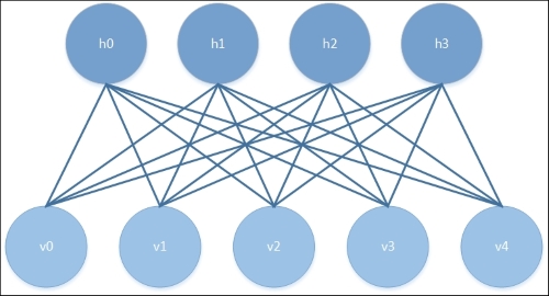
One advantage of this topology is that the hidden and visible layers are conditionally independent given one another. As such, it is possible to sample from one layer using the activations of the other.

Now that we have a general working knowledge of the RBM algorithm, let's walk through code to create an RBM. We'll be working with an RBM class that will allow us to classify the MNIST handwritten digits dataset. The code we're about to review does the following:

Let's begin examining our RBM class:

class RBM(object):
    def __init__(
        self,
        input=None,
        n_visible=784,
        n_hidden=500,
        w=None,
        hbias=None,
        vbias=None,
        numpy_rng=None,
        theano_rng=None
    ):

The first element that we need to build is an RBM constructor, which we can use to define the parameters of the model, such as the number of visible and hidden nodes (n_visible and n_hidden) as well as additional parameters that can be used to adjust how the RBM's inference functions and CD updates are performed.

The w parameter can be used as a pointer to a shared weight matrix. This becomes more relevant when implementing a DBN, as we'll see later in the chapter; in such architectures, the weight matrix needs to be shared between different parts of the network.

The hbias and vbias parameters are used similarly as optional references to shared hidden and visible (respectively) units' bias vectors. Again, these are used in DBNs.

The input parameter enables the RBM to be connected, top-to-tail, to other graph elements. This allows one to, for instance, chain RBMs.

Having set up this constructor, we next need to flesh out each of the preceding parameters:

        self.n_visible = n_visible
        self.n_hidden = n_hidden

        if numpy_rng is None:
            numpy_rng = numpy.random.RandomState(1234)

        if theano_rng is None:
            theano_rng = RandomStreams(numpy_rng.randint(2 ** 30))

This is fairly straightforward stuff; we set the visible and hidden nodes for our RBM and set up two random number generators. The theano_rng parameter will be used later in our code to sample from the RBM's hidden units:

        if W is None:
            initial_W = numpy.asarray(
                numpy_rng.uniform(
                    low=-4 * numpy.sqrt(6. / (n_hidden + n_visible)),
                    high=4 * numpy.sqrt(6. / (n_hidden + n_visible)),
                    size=(n_visible, n_hidden)
                ),
                dtype=theano.config.floatX
            )

This code switches up the data type for W so that it can be run over the GPU. Next, we set up shared variables using theano.shared, which allows a variable's storage to be shared between functions that it appears in. Within the current example, the shared variables that we create will be the weight vector (W) and bias variables for hidden and visible units (hbias and vbias, respectively). When we move on to creating deep networks with multiple components, the following code will allow us to share components between parts of our networks:

            W = theano.shared(value=initial_W, name='W', borrow=True)

        if hbias is None: 
            hbias = theano.shared(
                value=numpy.zeros(
                    n_hidden,
                    dtype=theano.config.floatX
                ),
                name='hbias',
                borrow=True
            )

        if vbias is None:
            vbias = theano.shared(
                value=numpy.zeros(
                    n_visible,
                    dtype=theano.config.floatX
                ),
                name='vbias',
                borrow=True
            )

At this point, we're ready to initialize the input layer as follows:

        self.input = input
        if not input:
            self.input = T.matrix('input')

        self.W = W
        self.hbias = hbias
        self.vbias = vbias
        self.theano_rng = theano_rng
        self.params = [self.W, self.hbias, self.vbias]

As we now have an initialized input layer, our next task is to create the symbolic graph that we described earlier in the chapter. Achieving this is a matter of creating functions to manage the interlayer propagation and activation computation operations of the network:

def propup(self, vis):
        pre_sigmoid_activation = T.dot(vis, self.W) + self.hbias
        return [pre_sigmoid_activation, T.nnet.sigmoid(pre_sigmoid_activation)]


    def propdown(self, hid):
        pre_sigmoid_activation = T.dot(hid, self.W.T) + self.vbias
        return [pre_sigmoid_activation, T.nnet.sigmoid(pre_sigmoid_activation)]

These two functions pass the activation of one layer's units to the other layer. The first function passes the visible units' activation upward to the hidden units so that the hidden units can compute their activation conditional on a sample of the visible units. The second function does the reverse—propagating the hidden layer's activation downward to the visible units.

It's probably worth asking why we're creating both propup and propdown. As we reviewed it, PCD only requires that we perform sampling from the hidden units. So what's the value of propup?

In a nutshell, sampling from the visible layer becomes useful when we want to sample from the RBM to review its progress. In most applications where our RBM is processing visual data, it is immediately valuable to periodically take the output of sampling from the visible layer and plot it, as shown in the following example:

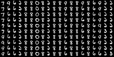
As we can see here, over the course of iteration, our network begins to change its labeling; in the first case, 7 morphs into 9, while elsewhere 9 becomes 6 and the network gradually reaches a definition of 3-ness.

As we discussed earlier, it's helpful to have as many views on the operation of your RBM as possible to ensure that it's delivering meaningful results. Sampling from the outputs it generates is one way to improve this visibility.

Armed with information about the visible layer's activation, we can deliver a sample of the unit activations from the hidden layer, given the activation of the hidden nodes:

    def sample_h_given_v(self, v0_sample):
     
 pre_sigmoid_h1, h1_mean = self.propup(v0_sample)
    h1_sample = self.theano_rng.binomial(size=h1_mean.shape,
    n=1, p=h1_mean, dtype=theano.config.floatX)

    return [pre_sigmoid_h1, h1_mean, h1_sample]

Likewise, we can now sample from the visible layer given hidden unit activation information:

    def sample_v_given_h(self, h0_sample):
    pre_sigmoid_v1, v1_mean = self.propdown(h0_sample)
      v1_sample = self.theano_rng.binomial(size=v1_mean.shape,
      n=1, p=v1_mean, dtype=theano.config.floatX)

      return [pre_sigmoid_v1, v1_mean, v1_sample]

We've now achieved the connectivity and update loop required to perform a Gibbs sampling step, as described earlier in this chapter. Next, we should define this sampling step!

    def gibbs_hvh(self, h0_sample):
        
        pre_sigmoid_v1, v1_mean, v1_sample = 
        self.sample_v_given_h(h0_sample)
        pre_sigmoid_h1, h1_mean, h1_sample = 
        self.sample_h_given_v(v1_sample)
        return [pre_sigmoid_v1, v1_mean, v1_sample,
                pre_sigmoid_h1, h1_mean, h1_sample]

As discussed, we need a similar function to sample from the visible layer:

    def gibbs_vhv(self, v0_sample):
        
        pre_sigmoid_h1, h1_mean, h1_sample = 
        self.sample_h_given_v(v0_sample)
        pre_sigmoid_v1, v1_mean, v1_sample = 
        self.sample_v_given_h(h1_sample)
        return [pre_sigmoid_h1, h1_mean, h1_sample,
                pre_sigmoid_v1, v1_mean, v1_sample]

The code that we've written so far gives us some of our model. It set up the nodes and layers and connections between layers. We've written the code that we need in order to update the network based on Gibbs sampling from the hidden layer.

What we're still missing is code that allows us to perform the following:

First off, we'll create the means to calculate the free energy of our RBM. Note that this is the inverse log of the probability distribution for the hidden layer, which we discussed earlier:

  def free_energy(self, v_sample):
        
        wx_b = T.dot(v_sample, self.W) + self.hbias
        vbias_term = T.dot(v_sample, self.vbias)
        hidden_term = T.sum(T.log(1 + T.exp(wx_b)), axis=1)
        return -hidden_term - vbias_term

Next, we'll implement PCD. At this point, we'll be setting a couple of interesting parameters. The lr, short for learning rate, is an adjustable parameter used to adjust learning speed. The k parameter points to the number of steps to be performed by PCD (remember the PCD-k notation from earlier in the chapter?).

We discussed the PCD as containing two phases, positive and negative. The following code computes the positive phase of PCD:

def get_cost_updates(self, lr=0.1, persistent = , k=1):

        pre_sigmoid_ph, ph_mean, ph_sample =  
        self.sample_h_given_v(self.input)

        
       
            chain_start = persistent

Meanwhile, the following code implements the negative phase of PCD. To do so, we scan the gibbs_hvh function k times, using Theano's scan operation, performing one Gibbs sampling step with each scan. After completing the negative phase, we acquire the free energy value:

        (
            [
                pre_sigmoid_nvs,
                nv_means,
                nv_samples,
                pre_sigmoid_nhs,
                nh_means,
                nh_samples
            ],
            updates
        ) = theano.scan(
            self.gibbs_hvh,
            outputs_info=[None, None, None, None, None, chain_start],
            n_steps=k
        )


        chain_end = nv_samples[-1]

        cost = T.mean(self.free_energy(self.input)) - T.mean(
            self.free_energy(chain_end))

        gparams = T.grad(cost, self.params, 
        consider_constant=[chain_end])

Having written code that performs the full PCD process, we need a way to feed the outputs to our network. At this point, we're able to connect our PCD learning process to the code to update the network that we reviewed earlier. The preceding updates dictionary points to theano.scan of the gibbs_hvh function. As you may recall, gibbs_hvh currently contains rules for random states of theano_rng. What we need to do now is add the new parameter values and variable containing the state of the Gibbs chain to the dictionary (the updates variable):

        for gparam, param in zip(gparams, self.params):
            updates[param] = param - gparam * T.cast(
                lr,
                dtype=theano.config.floatX
            )
        
            updates = nh_samples[-1]
            monitoring_cost =  
            self.get_pseudo_likelihood_cost(updates)
        

        return monitoring_cost, updates

We now have almost all the parts that we need to make our RBM work. What's clearly missing is a means to inspect training, either during or after completion, to ensure that our RBM is learning an appropriate representation of the data.

We talked previously about how to train an RBM, specifically about challenges posed by the partition function. Furthermore, earlier in the code, we implemented one means by which we can inspect an RBM during training; we created the gibbs_vhv function to perform Gibbs sampling from the model.

In our previous discussion around how to validate an RBM, we discussed visually plotting the filters that the RBM has created. We'll review how this can be achieved shortly.

The final possibility is to use the inverse log of the PL as a more tractable proxy to the likelihood itself. Technically, the log-PL is the sum of the log-probabilities of each data point (each x) conditioned on all other data points. As discussed, this becomes too expensive with larger-dimensional datasets, so a stochastic approximation to log-PL is used.

We referenced a function that will enable us to get PL cost during the get_cost_updates function, specifically the get_pseudo_likelihood_cost function. Now it's time to flesh out this function and obtain the pseudo-likelihood:

def get_pseudo_likelihood_cost(self, updates):

        bit_i_idx = theano.shared(value=0, name='bit_i_idx')
        xi = T.round(self.input)

        fe_xi = self.free_energy(xi)

        xi_flip = T.set_subtensor(xi[:, bit_i_idx], 1 - xi[:, 
        bit_i_idx])

        fe_xi_flip = self.free_energy(xi_flip)

        cost = T.mean(self.n_visible * 
        T.log(T.nnet.sigmoid(fe_xi_flip - fe_xi)))

        
        updates[bit_i_idx] = (bit_i_idx + 1) % self.n_visible

        return cost

We've now filled out each element on the list of missing components and have completely reviewed the RBM class. We've explored how each element ties into the theory behind the RBM and should now have a thorough understanding of how the RBM algorithm works. We understand what the outputs of our RBM will be and will soon be able to review and assess them. In short, we're ready to train our RBM. Beginning the training of the RBM is a matter of running the following code, which triggers the train_set_x function. We'll discuss this function in greater depth later in this chapter:

    train_rbm = theano.function(
        [index],
        cost,
        updates=updates,
        givens={
            x: train_set_x[index * batch_size: (index + 1) * 
            batch_size]
        },
        name='train_rbm'
    )

    plotting_time = 0.
    start_time = time.clock()

Having updated the RBM's updates and training set, we run through training epochs. Within each epoch, we train over the training data before plotting the weights as a matrix (as described earlier in the chapter):

    for epoch in xrange(training_epochs):

        mean_cost = []
        for batch_index in xrange(n_train_batches):
            mean_cost += [train_rbm(batch_index)]

        print 'Training epoch %d, cost is ' % epoch, 
        numpy.mean(mean_cost)

        plotting_start = time.clock()
        image = Image.fromarray(
            tile_raster_images(
                X=rbm.W.get_value(borrow=True).T,
                img_shape=(28, 28),
                tile_shape=(10, 10),
                tile_spacing=(1, 1)
            )
        )
        image.save('filters_at_epoch_%i.png' % epoch)
        plotting_stop = time.clock()
        plotting_time += (plotting_stop - plotting_start)

    end_time = time.clock()

    pretraining_time = (end_time - start_time) - plotting_time

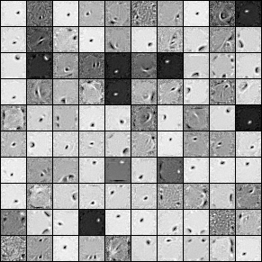
    print ('Training took %f minutes' % (pretraining_time / 60.))

The weights tend to plot fairly recognizably and resemble Gabor filters (linear filters commonly used for edge detection in images). If your dataset is handwritten characters on a fairly low-noise background, you tend to find that the weights trace the strokes used. For photographs, the filters will approximately trace edges in the image. The following image shows an example output:

Finally, we create the persistent Gibbs chains that we need to derive our samples. The following function performs a single Gibbs step, as discussed previously, then updates the chain:

plot_every = 1000

    (
        [
            presig_hids,
            hid_mfs,
            hid_samples,
            presig_vis,
            vis_mfs,
            vis_samples
        ],
        updates
    ) = theano.scan(
        rbm.gibbs_vhv,
        outputs_info=[None, None, None, None, None, persistent_vis_chain],
        n_steps=plot_every
    )

This code runs the gibbs_vhv function we described previously, plotting network output samples for our inspection:

    updates.update({persistent_vis_chain: vis_samples[-1]})
    sample_fn = theano.function(
        [],
        [
            vis_mfs[-1],
            vis_samples[-1]
        ],
        updates=updates,
        name='sample_fn'
    )

    image_data = numpy.zeros(
        (29 * n_samples + 1, 29 * n_chains - 1),
        dtype='uint8'
    )
    for idx in xrange(n_samples):
        
        vis_mf, vis_sample = sample_fn()
        print ' ... plotting sample ', idx
        image_data[29 * idx:29 * idx + 28, :] = tile_raster_images(
            X=vis_mf,
            img_shape=(28, 28),
            tile_shape=(1, n_chains),
            tile_spacing=(1, 1)
        )

    image = Image.fromarray(image_data)
    image.save('samples.png')

At this point, we have an entire RBM. We have the PCD algorithm and the ability to update the network using this algorithm and Gibbs sampling. We have several visible output methods so that we can assess how well our RBM has trained.

However, we're not done yet! Next, we'll begin to see what the most frequent and powerful application of the RBM is.

We can use the RBM as an ML algorithm in and of itself. It functions comparably well with other algorithms. Advantageously, it can be scaled up to a point where it can learn high-dimensional datasets. However, this isn't where the real strength of the RBM lies.

The RBM is most commonly used as a pretraining mechanism for a highly effective deep network architecture called a DBN. DBNs are extremely powerful tools to learn and classify a range of image datasets. They possess a very good ability to generalize to unknown cases and are among the best image-learning tools available. For this reason, DBNs are in use at many of the world's top tech and data science companies, primarily in image search and recognition contexts.