In order to import JSON-compliant files, we should first create a SQL context, creating a SQLContext object from the local Spark Context:

In:from pyspark.sql import SQLContext
sqlContext = SQLContext(sc)

Now, let's see the content of a small JSON file (it's provided in the Vagrant virtual machine). It's a JSON representation of a table with six rows and three columns, where some attributes are missing (such as the gender attribute for the user with user_id=0):

In:!cat /home/vagrant/datasets/users.json

Out:{"user_id":0, "balance": 10.0}
{"user_id":1, "gender":"M", "balance": 1.0}
{"user_id":2, "gender":"F", "balance": -0.5}
{"user_id":3, "gender":"F", "balance": 0.0}
{"user_id":4, "balance": 5.0}
{"user_id":5, "gender":"M", "balance": 3.0}

Using the read.json method provided by sqlContext, we already have the table well formatted and with all the right column names in a variable. The output variable is typed as Spark DataFrame. To show the variable in a nice, formatted table, use its show method:

In:
df = sqlContext.read 
.json("file:///home/vagrant/datasets/users.json")
df.show()

Out:
+-------+------+-------+
|balance|gender|user_id|
+-------+------+-------+
|   10.0|  null|      0|
|    1.0|     M|      1|
|   -0.5|     F|      2|
|    0.0|     F|      3|
|    5.0|  null|      4|
|    3.0|     M|      5|
+-------+------+-------+

Additionally, we can investigate the schema of the DataFrame using the printSchema method. We realize that, while reading the JSON file, each column type has been inferred by the data (in the example, the user_id column contains long integers, the gender column is composed by strings, and the balance is a double floating point):

In:df.printSchema()

Out:root
 |-- balance: double (nullable = true)
 |-- gender: string (nullable = true)
 |-- user_id: long (nullable = true)

Exactly like a table in an RDBMS, we can slide and dice the data in the DataFrame, making selections of columns and filtering the data by attributes. In this example, we want to print the balance, gender, and user_id of the users whose gender is not missing and have a balance strictly greater than zero. For this, we can use the filter and select methods:

In:(df.filter(df['gender'] != 'null')
.filter(df['balance'] > 0)
   .select(['balance', 'gender', 'user_id'])
   .show())

Out:
+-------+------+-------+
|balance|gender|user_id|
+-------+------+-------+
|    1.0|     M|      1|
|    3.0|     M|      5|
+-------+------+-------+

We can also rewrite each piece of the preceding job in a SQL-like language. In fact, filter and select methods can accept SQL-formatted strings:

In:(df.filter('gender is not null')
   .filter('balance > 0').select("*").show())

Out:
+-------+------+-------+
|balance|gender|user_id|
+-------+------+-------+
|    1.0|     M|      1|
|    3.0|     M|      5|
+-------+------+-------+

We can also use just one call to the filter method:

In:df.filter('gender is not null and balance > 0').show()

Out:
+-------+------+-------+
|balance|gender|user_id|
+-------+------+-------+
|    1.0|     M|      1|
|    3.0|     M|      5|
+-------+------+-------+

A common problem of data preprocessing is to handle missing data. Spark DataFrames, similar to pandas DataFrames, offer a wide range of operations that you can do on them. For example, the easiest option to have a dataset composed by complete rows only is to discard rows containing missing information. For this, in a Spark DataFrame, we first have to access the na attribute of the DataFrame and then call the drop method. The resulting table will contain only the complete rows:

In:df.na.drop().show()

Out:
+-------+------+-------+
|balance|gender|user_id|
+-------+------+-------+
|    1.0|     M|      1|
|   -0.5|     F|      2|
|    0.0|     F|      3|
|    3.0|     M|      5|
+-------+------+-------+

If such an operation is removing too many rows, we can always decide what columns should be accounted for the removal of the row (as the augmented subset of the drop method):

In:df.na.drop(subset=["gender"]).show()

Out:
+-------+------+-------+
|balance|gender|user_id|
+-------+------+-------+
|    1.0|     M|      1|
|   -0.5|     F|      2|
|    0.0|     F|      3|
|    3.0|     M|      5|
+-------+------+-------+

Also, if you want to set default values for each column instead of removing the line data, you can use the fill method, passing a dictionary composed by the column name (as the dictionary key) and the default value to substitute missing data in that column (as the value of the key in the dictionary).

As an example, if you want to ensure that the variable balance, where missing, is set to 0, and the variable gender, where missing, is set to U, you can simply do the following:

In:df.na.fill({'gender': "U", 'balance': 0.0}).show()

Out:
+-------+------+-------+
|balance|gender|user_id|
+-------+------+-------+
|   10.0|     U|      0|
|    1.0|     M|      1|
|   -0.5|     F|      2|
|    0.0|     F|      3|
|    5.0|     U|      4|
|    3.0|     M|      5|
+-------+------+-------+

To have a function applied on a group of rows (exactly as in the case of SQL GROUP BY), you can use two similar methods. In the following example, we want to compute the average balance per gender:

In:(df.na.fill({'gender': "U", 'balance': 0.0})
   .groupBy("gender").avg('balance').show())

Out:
+------+------------+
|gender|avg(balance)|
+------+------------+
|     F|       -0.25|
|     M|         2.0|
|     U|         7.5|
+------+------------+

So far, we've worked with DataFrames but, as you've seen, the distance between DataFrame methods and SQL commands is minimal. Actually, using Spark, it is possible to register the DataFrame as a SQL table to fully enjoy the power of SQL. The table is saved in-memory and distributed in a way similar to an RDD.

To register the table, we need to provide a name, which will be used in future SQL commands. In this case, we decide to name it users:

In:df.registerTempTable("users")

By calling the sql method provided by the Spark sql context, we can run any SQL-compliant table:

In:sqlContext.sql("""
    SELECT gender, AVG(balance) 
    FROM users 
    WHERE gender IS NOT NULL 
    GROUP BY gender""").show()

Out:
+------+-----+
|gender|  _c1|
+------+-----+
|     F|-0.25|
|     M|  2.0|
+------+-----+

Not surprisingly, the table outputted by the command (as well as the users table itself) is of the Spark DataFrame type:

In:type(sqlContext.table("users"))

Out:pyspark.sql.dataframe.DataFrame

DataFrames, tables, and RDDs are intimately connected, and RDD methods can be used on a DataFrame. Remember that each row of the DataFrame is an element of the RDD. Let's see this in detail and first collect the whole table:

In:sqlContext.table("users").collect()
Out:[Row(balance=10.0, gender=None, user_id=0),
 Row(balance=1.0, gender=u'M', user_id=1),
 Row(balance=-0.5, gender=u'F', user_id=2),
 Row(balance=0.0, gender=u'F', user_id=3),
 Row(balance=5.0, gender=None, user_id=4),
 Row(balance=3.0, gender=u'M', user_id=5)]

In:
a_row = sqlContext.sql("SELECT * FROM users").first()
a_row

Out:Row(balance=10.0, gender=None, user_id=0)

The output is a list of Row objects (they look like Python's namedtuple). Let's dig deeper into it: Row contains multiple attributes, and it's possible to access them as a property or dictionary key; that is, to have the balance out from the first row, we can choose between the two following ways:

In:print a_row['balance']
print a_row.balance

Out:10.0
10.0

Also, Row can be collected as a Python dictionary using the asDict method of Row. The result contains the property names as a key and property values as dictionary values:

In:a_row.asDict()

Out:{'balance': 10.0, 'gender': None, 'user_id': 0}

To write a DataFrame or RDD to disk, we can use the write method. We have a selection of formats; in this case, we will save it as a JSON file on the local machine:

In:(df.na.drop().write
   .save("file:///tmp/complete_users.json", format='json'))

Checking the output on the local filesystem, we immediately see that something is different from what we expected: this operation creates multiple files (part-r-…).

Each of them contains some rows serialized as JSON objects, and merging them together will create the comprehensive output. As Spark is made to process large and distributed files, the write operation is tuned for that and each node writes part of the full RDD:

In:!ls -als /tmp/complete_users.json

Out:total 28
4 drwxrwxr-x 2 vagrant vagrant 4096 Feb 25 22:54 .
4 drwxrwxrwt 9 root    root    4096 Feb 25 22:54 ..
4 -rw-r--r-- 1 vagrant vagrant   83 Feb 25 22:54 part-r-00000-...
4 -rw-rw-r-- 1 vagrant vagrant   12 Feb 25 22:54 .part-r-00000-...
4 -rw-r--r-- 1 vagrant vagrant   82 Feb 25 22:54 part-r-00001-...
4 -rw-rw-r-- 1 vagrant vagrant   12 Feb 25 22:54 .part-r-00001-...
0 -rw-r--r-- 1 vagrant vagrant    0 Feb 25 22:54 _SUCCESS
4 -rw-rw-r-- 1 vagrant vagrant    8 Feb 25 22:54 ._SUCCESS.crc

In order to read it back, we don't have to create a standalone file—even multiple pieces are fine in the read operation. A JSON file can also be read in the FROM clause of a SQL query. Let's now try to print the JSON that we've just written on disk without creating an intermediate DataFrame:

In:sqlContext.sql(
    "SELECT * FROM json.`file:///tmp/complete_users.json`").show()

Out:
+-------+------+-------+
|balance|gender|user_id|
+-------+------+-------+
|    1.0|     M|      1|
|   -0.5|     F|      2|
|    0.0|     F|      3|
|    3.0|     M|      5|
+-------+------+-------+

Beyond JSON, there is another format that's very popular when dealing with structured big datasets: Parquet format. Parquet is a columnar storage format that's available in the Hadoop ecosystem; it compresses and encodes the data and can work with nested structures: all such qualities make it very efficient.

Saving and loading is very similar to JSON and, even in this case, this operation produces multiple files written to disk:

In:df.na.drop().write.save(
    "file:///tmp/complete_users.parquet", format='parquet')

In:!ls -als /tmp/complete_users.parquet/

Out:total 44
4 drwxrwxr-x  2 vagrant vagrant 4096 Feb 25 22:54 .
4 drwxrwxrwt 10 root    root    4096 Feb 25 22:54 ..
4 -rw-r--r--  1 vagrant vagrant  376 Feb 25 22:54 _common_metadata
4 -rw-rw-r--  1 vagrant vagrant   12 Feb 25 22:54 ._common_metadata..
4 -rw-r--r--  1 vagrant vagrant 1082 Feb 25 22:54 _metadata
4 -rw-rw-r--  1 vagrant vagrant   20 Feb 25 22:54 ._metadata.crc
4 -rw-r--r--  1 vagrant vagrant  750 Feb 25 22:54 part-r-00000-...
4 -rw-rw-r--  1 vagrant vagrant   16 Feb 25 22:54 .part-r-00000-...
4 -rw-r--r--  1 vagrant vagrant  746 Feb 25 22:54 part-r-00001-...
4 -rw-rw-r--  1 vagrant vagrant   16 Feb 25 22:54 .part-r-00001-...
0 -rw-r--r--  1 vagrant vagrant    0 Feb 25 22:54 _SUCCESS
4 -rw-rw-r--  1 vagrant vagrant    8 Feb 25 22:54 ._SUCCESS.crc

So far, we've described how to load DataFrames from JSON and Parquet files, but not how to create them from an existing RDD. In order to do so, you just need to create one Row object for each record in the RDD and call the createDataFrame method of the SQL context. Finally, you can register it as a temp table to use the power of the SQL syntax fully:

In:from pyspark.sql import Row

rdd_gender = 
    sc.parallelize([Row(short_gender="M", long_gender="Male"),
                    Row(short_gender="F", long_gender="Female")])

(sqlContext.createDataFrame(rdd_gender)
           .registerTempTable("gender_maps"))

In:sqlContext.table("gender_maps").show()

Out:
+-----------+------------+
|long_gender|short_gender|
+-----------+------------+
|       Male|           M|
|     Female|           F|
+-----------+------------+

When you have multiple DataFrames in-memory, or that can be loaded from disk, you can join and use all the operations available in a classic RDBMS. In this example, we can join the DataFrame we've created from the RDD with the users dataset contained in the Parquet file that we've stored. The result is astonishing:

In:sqlContext.sql("""
    SELECT balance, long_gender, user_id 
    FROM parquet.`file:///tmp/complete_users.parquet` 
    JOIN gender_maps ON gender=short_gender""").show()

Out:
+-------+-----------+-------+
|balance|long_gender|user_id|
+-------+-----------+-------+
|    3.0|       Male|      5|
|    1.0|       Male|      1|
|    0.0|     Female|      3|
|   -0.5|     Female|      2|
+-------+-----------+-------+

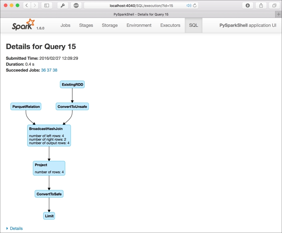
In the web UI, each SQL query is mapped as a virtual directed acyclic graph (DAG) under the SQL tab. This is very nice to keep track of the progress of your job and understand the complexity of the query. While doing the preceding JOIN query, you can clearly see that two branches are entering the same BroadcastHashJoin block: the first one is from an RDD and the second one is from a Parquet file. Then, the following block is simply a projetion on the selected columns:

As the tables are in-memory, the last thing to do is to clean up releasing the memory used to keep them. By calling the tableNames method, provided by the sqlContext, we have the list of all the tables that we currently have in-memory. Then, to free them up, we can use dropTempTable with the name of the table as argument. Beyond this point, any further reference to these tables will return an error:

In:sqlContext.tableNames()

Out:[u'gender_maps', u'users']

In:
for table in sqlContext.tableNames():
    sqlContext.dropTempTable(table)

Since Spark 1.3, DataFrame is the preferred way to operate on a dataset when doing data science operations.