 Extracting learning curves
by Alberto Boschetti, Luca Massaron, Bastiaan Sjardin, John Hearty, Prateek Joshi
Python: Real World Machine Learning
Extracting learning curves
by Alberto Boschetti, Luca Massaron, Bastiaan Sjardin, John Hearty, Prateek Joshi
Python: Real World Machine Learning
- Python: Real World Machine Learning
- Table of Contents
- Python: Real World Machine Learning
- Python: Real World Machine Learning
- Credits
- Preface
- I. Module 1
- 1. The Realm of Supervised Learning
- Introduction
- Preprocessing data using different techniques
- Label encoding
- Building a linear regressor
- Computing regression accuracy
- Achieving model persistence
- Building a ridge regressor
- Building a polynomial regressor
- Estimating housing prices
- Computing the relative importance of features
- Estimating bicycle demand distribution
- 2. Constructing a Classifier
- Introduction
- Building a simple classifier
- Building a logistic regression classifier
- Building a Naive Bayes classifier
- Splitting the dataset for training and testing
- Evaluating the accuracy using cross-validation
- Visualizing the confusion matrix
- Extracting the performance report
- Evaluating cars based on their characteristics
- Extracting validation curves
- Extracting learning curves
- Estimating the income bracket
- 3. Predictive Modeling
- 4. Clustering with Unsupervised Learning
- Introduction
- Clustering data using the k-means algorithm
- Compressing an image using vector quantization
- Building a Mean Shift clustering model
- Grouping data using agglomerative clustering
- Evaluating the performance of clustering algorithms
- Automatically estimating the number of clusters using DBSCAN algorithm
- Finding patterns in stock market data
- Building a customer segmentation model
- 5. Building Recommendation Engines
- Introduction
- Building function compositions for data processing
- Building machine learning pipelines
- Finding the nearest neighbors
- Constructing a k-nearest neighbors classifier
- Constructing a k-nearest neighbors regressor
- Computing the Euclidean distance score
- Computing the Pearson correlation score
- Finding similar users in the dataset
- Generating movie recommendations
- 6. Analyzing Text Data
- Introduction
- Preprocessing data using tokenization
- Stemming text data
- Converting text to its base form using lemmatization
- Dividing text using chunking
- Building a bag-of-words model
- Building a text classifier
- Identifying the gender
- Analyzing the sentiment of a sentence
- Identifying patterns in text using topic modeling
- 7. Speech Recognition
- 8. Dissecting Time Series and Sequential Data
- Introduction
- Transforming data into the time series format
- Slicing time series data
- Operating on time series data
- Extracting statistics from time series data
- Building Hidden Markov Models for sequential data
- Building Conditional Random Fields for sequential text data
- Analyzing stock market data using Hidden Markov Models
- 9. Image Content Analysis
- Introduction
- Operating on images using OpenCV-Python
- Detecting edges
- Histogram equalization
- Detecting corners
- Detecting SIFT feature points
- Building a Star feature detector
- Creating features using visual codebook and vector quantization
- Training an image classifier using Extremely Random Forests
- Building an object recognizer
- 10. Biometric Face Recognition
- Introduction
- Capturing and processing video from a webcam
- Building a face detector using Haar cascades
- Building eye and nose detectors
- Performing Principal Components Analysis
- Performing Kernel Principal Components Analysis
- Performing blind source separation
- Building a face recognizer using Local Binary Patterns Histogram
- 11. Deep Neural Networks
- Introduction
- Building a perceptron
- Building a single layer neural network
- Building a deep neural network
- Creating a vector quantizer
- Building a recurrent neural network for sequential data analysis
- Visualizing the characters in an optical character recognition database
- Building an optical character recognizer using neural networks
- 12. Visualizing Data
- 1. The Realm of Supervised Learning
- II. Module 2
- 1. Unsupervised Machine Learning
- 2. Deep Belief Networks
- 3. Stacked Denoising Autoencoders
- 4. Convolutional Neural Networks
- 5. Semi-Supervised Learning
- 6. Text Feature Engineering
- 7. Feature Engineering Part II
- 8. Ensemble Methods
- 9. Additional Python Machine Learning Tools
- A. Chapter Code Requirements
- III. Module 3
- 1. First Steps to Scalability
- 2. Scalable Learning in Scikit-learn
- 3. Fast SVM Implementations
- 4. Neural Networks and Deep Learning
- The neural network architecture
- Neural networks and regularization
- Neural networks and hyperparameter optimization
- Neural networks and decision boundaries
- Deep learning at scale with H2O
- Deep learning and unsupervised pretraining
- Deep learning with theanets
- Autoencoders and unsupervised learning
- Summary
- 5. Deep Learning with TensorFlow
- 6. Classification and Regression Trees at Scale
- 7. Unsupervised Learning at Scale
- 8. Distributed Environments – Hadoop and Spark
- 9. Practical Machine Learning with Spark
- A. Introduction to GPUs and Theano
- A. Bibliography
- Index
Learning curves help us understand how the size of our training dataset influences the machine learning model. This is very useful when you have to deal with computational constraints. Let's go ahead and plot the learning curves by varying the size of our training dataset.
- Add the following code to the same Python file, as in the previous recipe:
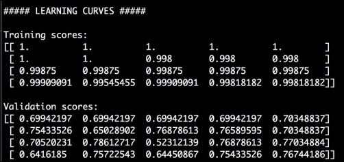
# Learning curves

from sklearn.learning_curve import learning_curve

classifier = RandomForestClassifier(random_state=7)

parameter_grid = np.array([200, 500, 800, 1100])
train_sizes, train_scores, validation_scores = learning_curve(classifier,
        X, y, train_sizes=parameter_grid, cv=5)
print "
##### LEARNING CURVES #####"
print "
Training scores:
", train_scores
print "
Validation scores:
", validation_scores
We want to evaluate the performance metrics using training datasets of size 200, 500, 800, and 1100. We use five-fold cross-validation, as specified by the
cvparameter in thelearning_curvemethod. - If you run this code, you will get the following output on the Terminal:
- Let's plot it:
# Plot the curve plt.figure() plt.plot(parameter_grid, 100*np.average(train_scores, axis=1), color='black') plt.title('Learning curve') plt.xlabel('Number of training samples') plt.ylabel('Accuracy') plt.show() - Here is the output figure:
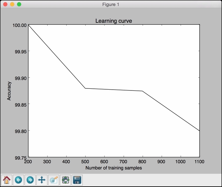
Although smaller training sets seem to give better accuracy, they are prone to overfitting. If we choose a bigger training dataset, it consumes more resources. Therefore, we need to make a trade-off here to pick the right size of the training dataset.
-
No Comment
..................Content has been hidden....................
You can't read the all page of ebook, please click here login for view all page.