
The goal of text classification is to categorize text documents into different classes. This is an extremely important analysis technique in NLP. We will use a technique, which is based on a statistic called tf-idf, which stands for term frequency—inverse document frequency. This is an analysis tool that helps us understand how important a word is to a document in a set of documents. This serves as a feature vector that's used to categorize documents. You can learn more about it at http://www.tfidf.com.
- Create a new Python file, and import the following package:
from sklearn.datasets import fetch_20newsgroups
- Let's select a list of categories and name them using a dictionary mapping. These categories are available as part of the news groups dataset that we just imported:
category_map = {'misc.forsale': 'Sales', 'rec.motorcycles': 'Motorcycles', 'rec.sport.baseball': 'Baseball', 'sci.crypt': 'Cryptography', 'sci.space': 'Space'} - Load the training data based on the categories that we just defined:
training_data = fetch_20newsgroups(subset='train', categories=category_map.keys(), shuffle=True, random_state=7) - Import the feature extractor:
# Feature extraction
from sklearn.feature_extraction.text import CountVectorizer
- Extract the features using the training data:
vectorizer = CountVectorizer()
X_train_termcounts = vectorizer.fit_transform(training_data.data)
print "
Dimensions of training data:", X_train_termcounts.shape
- We are now ready to train the classifier. We will use the Multinomial Naive Bayes classifier:
# Training a classifier
from sklearn.naive_bayes import MultinomialNB
from sklearn.feature_extraction.text import TfidfTransformer
- Define a couple of random input sentences:
input_data = [ "The curveballs of right handed pitchers tend to curve to the left", "Caesar cipher is an ancient form of encryption", "This two-wheeler is really good on slippery roads" ] - Define the tf-idf transformer object and train it:
# tf-idf transformer
tfidf_transformer = TfidfTransformer()
X_train_tfidf = tfidf_transformer.fit_transform(X_train_termcounts)
- Once we have the feature vectors, train the Multinomial Naive Bayes classifier using this data:
# Multinomial Naive Bayes classifier
classifier = MultinomialNB().fit(X_train_tfidf, training_data.target)
- Transform the input data using the word counts:
X_input_termcounts = vectorizer.transform(input_data)
- Transform the input data using the tf-idf transformer:
X_input_tfidf = tfidf_transformer.transform(X_input_termcounts)
- Predict the output categories of these input sentences using the trained classifier:
# Predict the output categories
predicted_categories = classifier.predict(X_input_tfidf)
- Print the outputs, as follows:
# Print the outputs for sentence, category in zip(input_data, predicted_categories): print ' Input:', sentence, ' Predicted category:', category_map[training_data.target_names[category]] - The full code is in the
tfidf.pyfile. If you run this code, you will see the following output printed on your Terminal: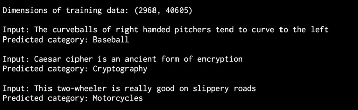
The tf-idf technique is used frequently in information retrieval. The goal is to understand the importance of each word within a document. We want to identify words that are occur many times in a document. At the same time, common words like “is” and “be” don't really reflect the nature of the content. So we need to extract the words that are true indicators. The importance of each word increases as the count increases. At the same time, as it appears a lot, the frequency of this word increases too. These two things tend to balance each other out. We extract the term counts from each sentence. Once we convert this to a feature vector, we train the classifier to categorize these sentences.
The term frequency (TF) measures how frequently a word occurs in a given document. As multiple documents differ in length, the numbers in the histogram tend to vary a lot. So, we need to normalize this so that it becomes a level playing field. To achieve normalization, we divide term-frequency by the total number of words in a given document. The inverse document frequency (IDF) measures the importance of a given word. When we compute TF, all words are considered to be equally important. To counter-balance the frequencies of commonly-occurring words, we need to weigh them down and scale up the rare ones. We need to calculate the ratio of the number of documents with the given word and divide it by the total number of documents. IDF is calculated by taking the negative algorithm of this ratio.
For example, simple words, such as "is" or "the" tend to appear a lot in various documents. However, this doesn't mean that we can characterize the document based on these words. At the same time, if a word appears a single time, this is not useful either. So, we look for words that appear a number of times, but not so much that they become noisy. This is formulated in the tf-idf technique and used to classify documents. Search engines frequently use this tool to order the search results by relevance.