
This is something that you will be really pleased to know about. Yes, Wireshark has made quite significant changes that will make your analytical tasks more comfortable. To understand the difference, the best option will be to go through an example.
We will try to create an IO graph in order to witness the changes that the new version has. I am using a capture file from the previous chapter, which has mixed packet types and mostly contains VoIP traffic. The sole purpose of this exercise is to see how graphs can be of better assistance in version 2 of Wireshark. Follow these steps to create an IO graph in Wireshark version 2.0:
- Capture the normal traffic from your network or open any previously captured trace file that you have.
- Click on IO Graph under Statistics. Once you do that, you will be directly presented with a graph without any further hassle:
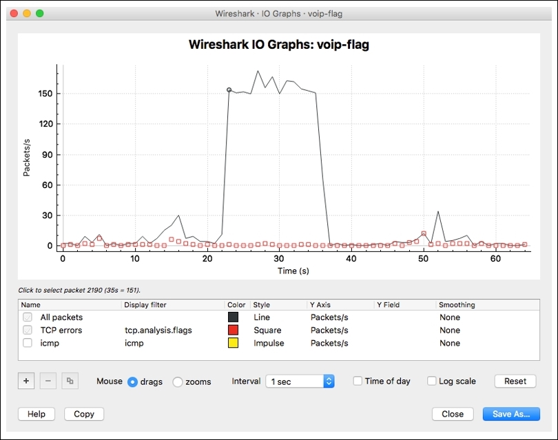
Figure 9.11: The IO graph
- Now, if you want to modify and configure the graph, then you can use various configurable options given at the bottom of the dialog.
- For instance, if I want to add any filter to the graph, I can click on the + symbol at the bottom and a new line will be shown, as in the following screenshot:
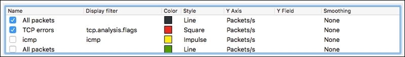
Figure 9.12: Adding a filter to a graph
- Now, I want to see the traffic pattern for the ARP packets along with other traffic-related details. So, I would write
arpas a filter expression in the display filter column and ARP packets in the name column. If you want to customize the look and feel too, you are most welcome to do so.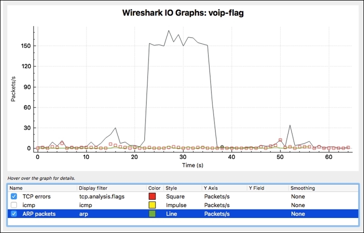
Figure 9.13: The ARP filter added in the IO graph
- As you can see, our newly created filter is in effect, and we can observe the frequency of ARP packets appearing in our graph as well.
Using graphs is now much more convenient, as you are no longer required to pass any statistical information to the graph. Just choose whichever graph you want, and then the default version of the graph will be presented to you without any questions asked. Now, if you feel like changing the graph as per your need, then just use the toolset given at the end of the graph to custom configure it.
Now, after we have made an IO graph, you will see how clean it looks; there are lots of features that have been introduced. Using the default graph, most of the time you will be able to figure out the ups and downs in your trace file. The legends are shown at the bottom most in a separate section, along with other configurable options like changing colors, hiding or enabling a filter, and much more.
Additional features can be listed and explored in the graphs; all you need to do is right-click on the graph area. The graph can now be moved along with the x and y axis by just clicking and dragging. Adding new arguments to the graph couldn't be any easier than this. As you can see, so many new amazing features are waiting for you to discover them.
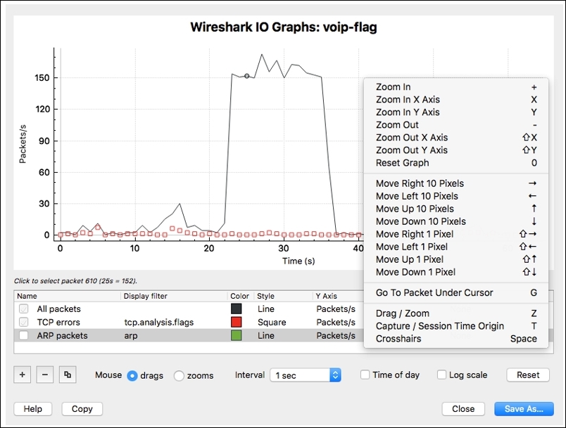
Figure 9.14: The right-click options list
Opening two graphs is now possible; and maybe someday, you will feel like comparing the traffic patterns in two trace files that you have. For example, I want to compare the normal VoIP traffic pattern and the malicious traffic pattern. Then, we can use two graphs to figure out the difference graphically, and it's really effective. Refer to the following screenshots:
Figure 9.15: Comparing two graphs at a single instance
Similarly, you can create a flow graph that can be of great assistance while analyzing the TCP flow and to know how SYN and ACK coordinate with each other. I would highly recommend that you create the flow graph in the newer version of Wireshark.
To switch between the graphs, you have the drop-down list sitting at the bottom-left corner of the graph window, which can assist you in doing so, and you are no longer required to go the window in the background to switch between graphs.
Another useful feature that can be taken advantage of when you are trying to create reports for your client or maybe for your own reference purpose is to export the graphs in PDF formats. You might have done this before; if not, then let's do this together here. Follow the given steps to do so:
- You need to click on the Save as icon at the bottom-right corner in the graph dialog window. Now, choose the location where you want to save the PDFs and click on Save.
- Once this has been done, you can export the PDF to anywhere you want to. Refer to the following screenshot:
Figure 9.16: Exporting graphs to PDF format
Now, whenever you want to import it into your report, just add it like an image and the graph from the PDF you exported will be added to your document. Doing this is really this easy:
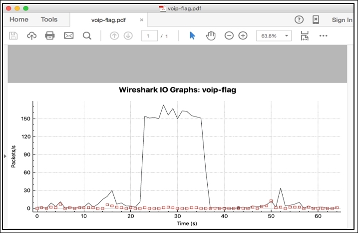
Figure 9.17: The graph exported as PDF