
Analyzing an application's performance problem is basically a case of identifying where the majority of the time for a particular task to complete is being spent, and measuring/comparing that time to what is normal and/or acceptable for that type of task.
Generally speaking, performance issues can be attributed to one of the following five areas, in order of decreasing likelihood:
- Server processing time delay
- Application turns delay
- Network path latency
- Bandwidth congestion
- Data transport (TCP) issues
Client processing time is usually a relatively small component of overall response time—except perhaps for some compute-extensive desktop applications, which leaves the focus on the network and server environments and any performance-affecting application design characteristics.
As was done when preparing to troubleshoot a connectivity or functionality problem, you'll need to gather the right information about the application environment and problem domain. You'll also want to determine which tools you may need to use during the analysis: Wireshark, TAPs to facilitate packet captures, and any other analysis tools.
You will also need to determine where to perform the first packet capture:
- A client-side capture is the best place to begin a performance analysis effort. From this vantage point, you can view and verify what the user is complaining about, view any error messages presented to the user or evident in the packet capture, measure network round-trip times, and capture the performance characteristics to study within a packet capture without the need to use a capture filter so you know you won't miss anything.
- A server-side capture may be needed because a client-side capture may not be possible for a user that is at a long distance, or to analyze server-to-server transactions to backend databases or other data sources.
- A packet capture at some intermediate point in the network path may be needed to isolate the source of excessive packet loss/errors and the associated retransmissions.
Remember that the use of an aggregating TAP is preferable over using SPAN ports, or you can install Wireshark on the client workstation or server as a last resort, but get the capture done any way you have to.
After performing the capture and saving the bulk capture file, confirm the following:
- Check the file to ensure there are no packets with the ACKed Unseen Segment messages in the Wireshark Warnings tab in the Expert Info menu, which means Wireshark saw a packet that was acknowledged but didn't see the original packet; an indication that Wireshark is missing packets due to a bad TAP or SPAN port configuration or excessive traffic levels. In any case, if more than just a few of these show up, you'll want to do the capture again after confirming the capture setup.
- Next, you'll want to review the captured conversations in IPv4 in the Conversations window and sort the Bytes column. The IP conversation between the user and application server should be at or near the top so you can select this conversation, right-click on it, and select A <-> B in the Selected menu.
- After reviewing the filtered data to ensure it contains what you expected, select Export Specified Packets from the File menu and save the filtered capture file with a filename that reflects the fact that this is a filtered subset of the bulk capture file.
- Finally, open the filtered file you just saved so you're working with a smaller, faster file without any distracting packets from other conversations that have nothing to do with your analysis.
At the onset of your analysis, you should take a look through the Errors, Warnings, and Notes tabs of Wireshark's Expert Info window (Analyze | Expert Info) for significant errors such as excessive retransmissions, Zero Window conditions, or application errors. These are very helpful to provide clues to the source of reported poor performance.
Although a few lost packets and retransmissions are normal and of minimal consequence in most packet captures, an excessive number indicates that network congestion is occurring somewhere in the path between user and server, packets are being discarded, and that an appreciable amount of time may be lost recovering from these lost packets.
Seeing a high count number of Duplicate ACK packets in the Expert Info Notes window may be alarming, but can be misleading. In the following screenshot, there was up to 69 Duplicate ACKs for one lost packet, and for a second lost packet the count went up to 89 (not shown in the following screenshot):

However, upon marking the time when the first Duplicate ACK occurred in Wireshark using the Set/Unset Time Reference feature in the Edit menu and then going to the last Duplicate ACK in this series by clicking the packet number in the Expert Info screen and inspecting a Relative time column in the Packet List pane, only 30 milliseconds had transpired. This is not a significant amount of time, especially if Selective Acknowledgment is enabled (as it was in this example) and other packets are being delivered and acknowledged in the meantime. Over longer latency network paths, the Duplicate ACK count can go much higher; it's only when the total number of lost packets and required retransmissions gets excessively high that the delay may become noticeable to a user.
Another condition to look for in the Expert Info Notes window includes the TCP Zero Window reports, which are caused by a receive buffer on the client or server being too full to accept any more data until the application has time to retrieve and process the data and make more room in the buffer. This isn't necessarily an error condition, but it can lead to substantial delays in transferring data, depending on how long it takes the buffer to get relieved.
You can measure this time by marking the TCP Zero Window packet with a time reference and looking at the elapsed relative time until a TCP Window Update packet is sent, which indicates the receiver is ready for more data. If this occurs frequently, or the delay between Zero Window and Window Update packets is long, you may need to inspect the host that is experiencing the full buffer condition to see whether there are any background processes that are adversely affecting the application that you're analyzing.
Note
If you haven't added them already, you need to add the Relative time and Delta time columns in the Packet List pane. Navigate to Edit | Preferences | Columns to add these. Adding time columns was also explained in Chapter 4, Configuring Wireshark.
You will probably see the connection reset (RST) messages in the Warnings tab. These are not indicators of an error condition if they occur at the end of a client-server exchange or session; they are normal indicators of sessions being terminated.
A very handy Filter Expression button you may want to add to Wireshark is a TCP Issues button using this display filter string as follows:
tcp.analysis.flags && !tcp.analysis.window_update && !tcp.analysis.keep_alive && !tcp.analysis.keep_alive_ack
This will filter and display most of the packets for which you will see the messages in the Expert Info window and provide a quick overview of any significant issues.
Since we're addressing application performance, the first step is to identify any delays in the packet flow so we can focus on the surrounding packets to identify the source and nature of the delay.
One of the quickest ways to identify delay events is to sort a TCP Delta time column (by clicking on the column header) so that the highest delay packets are arranged at the top of the packet list. You can then inspect the Info field of these packets to determine which, if any, reflect a valid performance affecting the event as most of them do not.
In the following screenshot, a TCP Delta time column is sorted in order of descending inter-packet times:
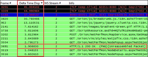
Let's have a detailed look at all the packets:
- The first two packets are the TCP Keep-Alive packets, which do just what they're called. They are a way for the client (or server) to make sure a connection is still alive (and not broken because the other end has gone away) after some time has elapsed with no activity. You can disregard these; they usually have nothing to do with the user experience.
- The third packet is a Reset packet, which is the last packet in the conversation stream and was sent to terminate the connection. Again, it has no impact on the user experience so you can ignore this.
- The next series of packets listed with a high inter-packet delay were GETs and a POST. These are the start of a new request and have occurred because the user clicked on a button or some other action on the application. However, the time that expired before these packets appear were consumed by the user think time—a period when the user was reading the last page and deciding what to do next. These also did not affect the user's response time experience and can be disregarded.
- Finally, Frame # 3691, which is a HTTP/1.1 200 OK, is a response from the server to a previous request; this is a legitimate response time of 1.9 seconds during which the user was waiting. If this response time had consumed more than a few seconds, the user may have grown frustrated with the wait and the type of request and reason for the excessive delay would warrant further analysis to determine why it took so long.
The point of this discussion is to illustrate that not all delays you may see in a packet trace affect the end user experience; you have to locate and focus on just those that do.
You may want to add some extra columns to Wireshark to speed up the analysis process; you can right-click on a column header and select Hide Column or Displayed Columns to show or hide specific columns:
- TCP Delta (tcp.time_delta): This is the time from one packet in a TCP conversation to the next packet in the same conversation/stream
- DNS Delta (dns.time): This is the time between DNS requests and responses
- HTTP Delta (http.time): This is the time between the HTTP requests and responses
While you're adding columns, the following can also be helpful during a performance analysis:
- Stream # (tcp.stream): This is the TCP conversation stream number. You can right-click on a stream number in this column, and select Selected from the Apply as a filter menu to quickly build a display filter to inspect a single conversation.
- Calc Win Size (tcp.window_size): This is the calculated TCP window size. This column can be used to quickly spot periods within a data delivery flow when the buffer size is decreasing to the point where a Zero Window condition occurred or almost occurred.
One of the most common causes of poor response times are excessively long server processing time events, which can be caused by processing times on the application server itself and/or delays incurred from long response times from a high number of requests to backend databases or other data sources.
Confirming and measuring these response times is easy within Wireshark using the following approach:
- Having used the sorted Delta Time column approach discussed in the previous section to identify a legitimate response time event, click on the suspect packet and then click on the Delta Time column header until it is no longer in the sort mode. This should result in the selected packet being highlighted in the middle of the Packet List pane and the displayed packets are back in their original order.
- Inspect the previous several packets to find the request that resulted in the long response time. The pattern that you'll see time and again is:
- The user sends a request to the server.
- The server fairly quickly acknowledges the request (with a [ACK] packet).
- After some time, the server starts sending data packets to service the request; the first of these packets is the packet you saw and selected in the sorted Delta Time view.
The time that expires between the first user request packet and the third packet when the server actually starts sending data is the First Byte response time. This is the area where you'll see longer response times caused by server processing time. This effect can be seen between users and servers, as well as between application servers and database servers or other data sources.
In the following screenshot, you can see a GET request from the client followed by an ACK packet from the server 198 milliseconds later (0.198651 seconds in the Delta Time Displ column); 1.9 seconds after that the server sends the first data packet (HTTP/1.1 200 OK in the Info field) followed by the start of a series of additional packets to deliver all of the requested data. In this illustration, a Time Reference has been set on the request packet. Looking at the Rel Time column, it can be seen that 2.107481 seconds transpired between the original request packet and the first byte packet:

It should be noted that how the First Byte data packet is summarized in the Info field depends upon the state of the Allow subdissector to reassemble TCP streams setting in the TCP menu, which can be found by navigating to Edit | Preferences | Protocols, as follows:
- If this option is disabled, the First Byte packet will display a summary of the contents of the first data packet in the Info field, such as HTTP/1.1 200 OK shown in the preceding screenshot, followed by a series of data delivery packets. The end of this delivery process has no remarkable signature; the packet flow just stops until the next request is received.
- If the Allow subdissector to reassemble TCP streams option is enabled, the First Byte packet will be summarized as simply a TCP segment of a reassembled PDU or similar notation. The HTTP/1.1 200 OK summary will be displayed in the Info field of the last data packet in this delivery process, signifying that the requested data has been delivered. An example of having this option enabled is illustrated in the following screenshot. This is the same request/response stream as shown in the preceding screenshot. It can be seen in the Rel Time column that the total elapsed time from the original request to the last data delivery packet was 2.1097 seconds:

In either case, the total response time as experienced by the user will be the time that transpires from the client request packet to the end of the data delivery packet plus the (usually) small amount of time required for the client application to process the received data and display the results on the user's screen.
In summary, measuring the time from the first request to the First Byte packets is the server response time. The time from the first request packet to the final data delivery packet is a good representation of the user response time experience.
The next, most likely source of poor response times—especially for remote users accessing applications over longer distances—is a relatively high number of what is known as application turns. An app turn is an instance where a client application makes a request and nothing else can or does happen until the response is received, after which another request/response cycle can occur, and so on.
Every client/server application is subject to the application turn effects and every request/response cycle incurs one. An application that imposes a high number of app turns to complete a task—due to poor application design, usually—can subject an end user to poor response times over higher latency network paths as the time spent waiting for these multiple requests and responses to traverse back and forth across the network adds up, which it can do quickly.
For example, if an application requires 100 application turns to complete a task and the round trip time (RTT) between the user and the application is 50 milliseconds (a typical cross-country value), the app turns delay will be 5 seconds:
100 App Turns X 50 ms RTT network latency = 5 seconds
This app turns' effect is additional wait (response) time on top of any server processing and network transport delays that is 5 seconds of totally wasted time. The resultant longer time inevitably gets blamed on the network; the network support teams assert that the network is working just fine and the application team points out that the application works fine until the network gets involved. And on it goes, so it is important to know about the app turns effects, what causes them, and how to measure and account for them.
Web applications can incur a relatively high app turn count due to the need to download one or more CSS files, JavaScript files, and multiple images to populate a page. Web designers can use techniques to reduce the app turn and download times, and modern browsers allow numerous connections to be used at the same time so that multiple requests can be serviced simultaneously, but the effects can still be significant over longer network paths. Many older, legacy applications and Microsoft's Server Message Block (SMB) protocols are also known to impose a high app turn count.
The presence and effects of application turns are not intuitively apparent in a packet capture unless you know they exist and how to identify and count them. You can do this in Wireshark for a client-side capture using a display filter:
ip.scr == 10.1.1.125 && tcp.analysis.ack_rtt > .008 && tcp.flags.ack == 1
You will need to replace the ip.src IP address with that of your server, and adjust the tcp.analysis.ack_rtt value to the RTT of the network path between the user and server. Upon applying the filter, you will see a display of packets that represent an application turn, and you can see the total app turns count in the Displayed field in the center section of the Wireshark's Status Bar option at the bottom of the user interface.
If you measure the total time required to complete a task (first request packet to last data delivery packet) and divide that time into the time incurred for application turns (number of app turns X network RTT), you can derive an approximate app turn time percentage:
5 seconds app turns delay / 7.5 seconds total response time = 66% of RT
Any percentage over 25 percent warrants further investigation into what can be done to reduce either the RTT latency (server placement) or the number app turns (application design).
The next leading cause of high response times is network path latency, which compounds the effects of application turns as discussed in the preceding section, as well as affecting data transport throughput and how long it takes to recover from packet loss and the subsequent retransmissions.
You can measure the network path latency between a client and server using the ICMP ping packets, but you can also determine this delay from a packet capture by measuring the time that transpires from a client SYN packet to the server's SYN, ACK response during a TCP three-way handshake process, as illustrated in the following figure of a client-side capture:

In a server-side capture, the time from the SYN, ACK to the client's ACK (third packet in the three-way handshake), also reflects the RTT. In practice, from any capture point, the time from the first SYN packet to the third ACK packet is a good representation of the RTT as well assuming the client and server response times during the handshake process are small. Be aware that the server response time to a SYN packet, while usually short, can be longer than normal during periods of high loading and can affect this measurement.
High network path latency isn't an error condition by itself, but can obviously have adverse effects on the application's operation over the network as previously discussed.
Bandwidth congestion affects the application's performance by extending the amount of time required to transmit a given amount of data over a network path; for users accessing an application server over a busy WAN link, these effects can become significant. A network support team should be able to generate bandwidth usage and availability reports for the in-path WAN links to check for this possibility, but you can also look for evidence of bandwidth congestion by using a properly configured Wireshark IO Graph to view network throughput during larger data transfers.
The following screenshot illustrates a data transfer that is affected by limited bandwidth; the flatlining at the 2.5 Mbps mark (the total bandwidth availability in this example), because no more bandwidth is available to support a faster transfer is clearly visible:
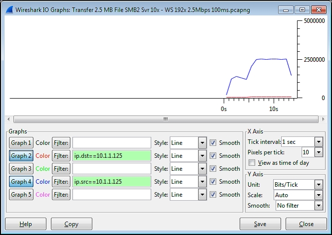
You can determine the peak data transfer rate in bits-per-second (bps) from an IO Graph by configuring the graph as follows:
- X Axis Tick interval: 1 sec
- Y Axis Unit: Bits/tick
- Graph 2 Filter:
ip.dst == <IP address of server> - Graph 4 Filter:
ip.src == <IP address of server>
These settings result in an accurate bits-per-second display of network throughput in client-to-server (red color) and server-to-client (blue color) directions. The Pixels per tick option in the X Axis panel, the Scale option in the Y Axis panel, and other settings can be modified as desired for the best display without affecting the accuracy of the measurement.
Be aware that most modern applications can generate short-term peak bandwidth demands (over an unrestricted link) of multiple Mbps. The WAN links along a network path should have enough spare capacity to accommodate these short term demands or response time will suffer accordingly. This is an important performance consideration.
There are a number of TCP data transport effects that can affect application performance; these can be analyzed in Wireshark.
Wireshark provides TCP StreamGraphs to analyze several key data transport metrics, including:
- Round-trip time: This graphs the RTT from a data packet to the corresponding ACK packet.
- Throughput: These are plots throughput in bytes per second.
- Time/sequence (Stephen's-style): This visualizes the TCP-based packet sequence numbers (and the number of bytes transferred) over time. An ideal graph flows from bottom-left to upper-right in a smooth fashion.
- Time/sequence (tcptrace): This is similar to the Stephen's graph, but provides more information. The data packets are represented with an I-bar display, where the taller the I-bar, the more data is being sent. A gray bar is also displayed that represents the receive window size. When the gray bar moves closer to the I-bars, the receive window size decreases.
- Window Scaling: This plots the receive window size.
These analysis graphs can be utilized by selecting one of the packets in a TCP stream in the Packet List pane and selecting TCP StreamGraph from the Statistics menu and then one of the options such as the Time-Sequence Graph (tcptrace).
The selected graph and Control Window will appear from the Graph type tab of the Control Window that you can select one of the other types of analysis graphs, as shown in the following screenshot:

The Time/Sequence Graph (tcptrace) shown in the following screenshot plots sequence numbers as they increase during a data transfer, along with the gray receive window size line:

You can click and drag the mouse over a section of the graph to zoom into a particular section, or press the + key to zoom in and the - key to zoom out. Clicking on a point in any of the graphs will take you to the corresponding packet in the Wireshark's Packet List pane.
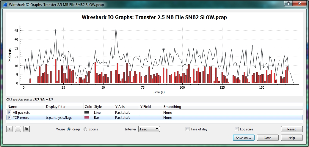
You can also analyze a the effects of TCP issues on network throughput by applying TCP analysis display filter strings to Wireshark's IO Graph, such as:
tcp.analysis.flags && !tcp.analysis.window_update
In the following screenshot of a slow SMB data transfer, it can be seen that the multiple TCP issues (in this case, packet loss, Duplicate ACKs, and retransmissions) in the red line correspond to a decrease in throughput (the black line):

Clicking on a point in the IO Graph takes you to the corresponding packet in the Wireshark's Packet List pane so you can investigate the issue.
Wireshark 2.0, also known as Wireshark Qt, is a major change in Wireshark's version history due to a transition from the GTK+ user interface library to Qt to provide better ongoing UI coverage for the supported platforms. Most of the Wireshark features and user interface controls will remain basically the same, but there are changes to the IO Graph.
These are shown in the following screenshot, which shows the same TCP issues that were seen in the preceding screenshot:
The new IO Graph window features the ability to add as many lines as desired (using the + key) and to zoom in on a graph line, as well as the ability to save the graph as an image or PDF document.