
In standard measurements with the IO Graph tool, we measure the performance of the network in units of packets/second, bytes/second, or bits/second. There are some types of data that cannot be measured with these parameters, and this is the reason we have the Advanced... feature in the Y-Axis options.
Choosing the Advanced... feature from the Unit: drop-down menu under Y-Axis opens a wider IO Graphs window, and provides the following options:
- SUM (*): This draws a graph with the summary of a parameter in the tick interval
- COUNT FRAMES (*): This draws a graph that counts the occurrence of the filtered frames in the tick interval
- COUNT FIELDS (*): This draws a graph that counts the occurrence of the filtered field in the tick interval
- MAX (*): This draws a graph with the maximum of a parameter in the tick interval
- MIN (*): This draws a graph with the minimum of a parameter in the tick interval
- AVG (*): This draws a graph with the average of a parameter in the tick interval
- LOAD (*): This is used for response time graphs
To start using the IO Graphs window with the Advanced feature, perform the following steps:
- Start the IO Graphs window from the Statistics menu.
- In the Unit: drop-down menu under Y-Axis, choose the Advanced… option. You will get the following window:

- You will see new drop-down menus with the string SUM(*).
- Choose SUM(*)/COUNT FRAMES (*)/COUNT FIELDS (*)/MAX(*)/MIN(*)/AVG(*)/ LOAD(*), and configure the appropriate filters. In the next recipes we will see some useful examples.
The time delta between frames can influence TCP performance, and there are cases in which we would like to correlate these with the performance we get from the network.
Let's look at the following capture file:

Here, we see packets sent from the source IP 10.2.10.105 as configured in the display filter.
To view the time variance between frames, configure the following parameters:
- To view the maximum
frame.time_deltavalue, configureip.src == 10.2.10.105in the field beside Filter: and choose MAX(*) and typeframe.time_deltain the fields beside Calc: - To view the average
frame.time_deltavalue, configureip.src == 10.2.10.105in the field beside Filter: and choose AVG(*) and typeframe.time_deltain the fields beside Calc: - To view the minimum
frame.time_deltavalue, configureip.src == 10.2.10.105in the field beside Filter: and choose MIN(*) and typeframe.time_deltain the fields beside Calc:
The graph that we will get is as follows:

What we see in the screenshot is a graph of the minimum, average, and maximum time delta between frames. What do we do with it and how do we use it for network debugging? This will be covered in Chapter 10, HTTP and DNS.
TCP events can be of many types: retransmissions, sliding window events, ACKs (or lack of them), and others. To see the number of TCP events over time, we can use the IO Graph tool with the Advanced... feature and the COUNT(*) parameter.
To do this, perform the following steps:
- Open IO Graphs from the Statistics menu.
- Under Y-Axis, choose Advanced... for Unit:.
- Configure the filters as follows:
- IP source and destination filters in the fields beside the Filter: buttons
- TCP events in the fields to the left of Style:
- Choose COUNT FRAMES (*) in the Calc: field and type
tcp.analysis.retransmissionsin the filter field
In this example, filters were configured to monitor TCP retransmissions on three different TCP streams.

In the graph of the preceding screenshot, you can see that retransmissions from each TCP stream are presented in different colors.
In various network protocols (mostly on those running over TCP), variations in time between frames (that is, the frame-time delta filter) can influence the performance significantly. One of the tools for viewing these changes in the IO Graphs window is the Advanced... configuration.
To do it, perform the following steps:
- Right-click on a packet in the suspicious TCP stream and navigate to Conversation filter | TCP. A filter will appear in the main filter box.
- Open IO Graph from the Statistics menu.
- Under Y-Axis, choose Advanced... for Unit:.
- Configure the filters as follows:
- Copy the filter definition from the upper filter box on the right-hand side to the IO Graph filter box on the left-hand side
- On the left-hand side, type the filter
frame.time_delta - Choose AVG(*) to see the average delta.
- Choose the appropriate X-Axis resolution.
Here is an example. In the following screenshot, we see a packet list with time variations between frames (a second time column was added in order to see the real time and time variations):
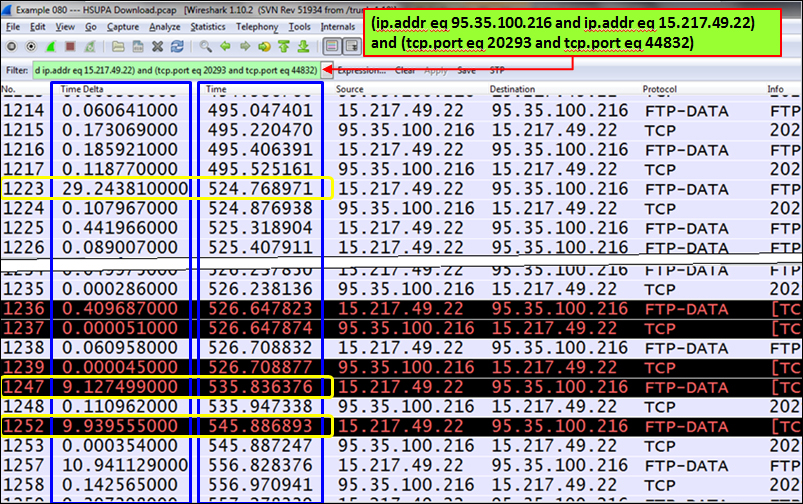
You see that there are some large time variations between frames; for example, 29.24 seconds in the frame 1,223, 9.12 seconds in the frame 1,247, and more.
In the IO Graphs window configured as described earlier, you will see the following:

As you see here, there are variations in time between frames. Later in this book, we will learn to see what causes these problems and how to solve them.
The IO Graph tool is one of the strongest and most efficient tools of Wireshark. While the standard IO Graph statistics can be used for basic statistics, the Advanced… feature can be used for in-depth monitoring of response times, TCP analysis of a single stream or several streams, and more.
When we configure a filter on the left, we will filter the traffic between hosts, traffic in a connection, traffic on a server, and so on. The Advanced… feature provides us with more details on traffic. Here are a few examples:
- On the left you see the TCP stream; on the right you see the time delta between frames in the stream
- On the left you see the video/RTP stream; on the right you see the occurrence of a marker bit