In this recipe we will learn how to use the IO Graph tool and how to configure it for network troubleshooting.
Under the Statistics menu, open the IO Graph tool by clicking on IO Graph. You can do this during an online file capture or on a file you've captured before. While using the IO Graph tool on a live capture, you will get live statistics on the captured data.
Run the IO Graph tool and you will get the following window:
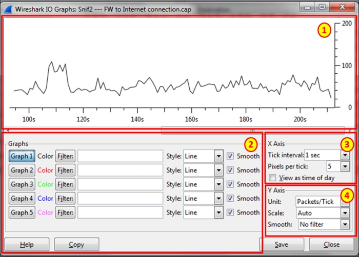
On the upper part of the window, you will get the graph highlighted as area 1. On the lower-left part, highlighted as area 2, you will get the filters that enable you to configure display filters, which will enable specific graphs. On the right-hand side of the window, highlighted as areas 3 and 4, you will get the X-Axis and Y-Axis configuration. Let's see what we can configure and how to do it.
- In the filter window, fill in a filter in the display-filter format. Only the packets that pass this filter will be taken into account for this graph. You have five optional filters to configure here.
- Choose the type of graph you want to present: Line, Impulse, FBar, or Dot.
- Click on the Graph button. This is required in order to activate the filter graph. Don't forget it.
- Choose a value to enter in Tick interval:. The scale can be between 0.001 seconds and 10 minutes.
Tip
If, for example, we get a peak of 1,000 packets/second when the tick interval X Axis is configured with 1-second intervals, it means that in the last second we've got 1,000 packets. When we change the tick interval for X Axis to 0.1-second intervals, the peak will be different because now we see how many packets were captured in the last 0.1 second.
- Choose the Pixels per tick: value to configure the pixels per tick interval.
- Mark the View as time of day button for choosing the time of day format instead of time since the beginning of capture.
- Choose the value for Unit: from Packets/Tick, Bytes/Tick, Bits/Tick, or Advanced... for choosing the Y-Axis scale.
- Choose Scale: for the Y Axis. You can choose it to be Linear or change it to Logarithmic. You can also leave it as Automatic or change it to manual values when required.
- Choose a value for Smooth: if you want to see a running average; that is, in every tick interval you will see the average of the past ticks. You can choose values from 4 to 1,024 to smooth the graph.
The IO Graphs feature is one of the important Wireshark tools that enable us to monitor online performance along with offline capture file analysis.
While you are using this tool, it's important to configure the right filter with the right X-Axis and Y-Axis parameters.
Let's have a look at the next two graphs, in which a PC with an IP address of 10.0.0.2 is browsing the Internet. In these two IO graphs, we have configured two filters:
- The first graph is the upload (upstream) traffic graph, which indicates all the traffic from the IP address 10.0.0.2; this is the filter
ip.src==10.0.0.2, colored in red. - The second graph is the download (downstream) traffic graph, which indicates all the traffic to the IP address 10.0.0.2; this is the filter
ip.dst==10.0.0.2, colored in green.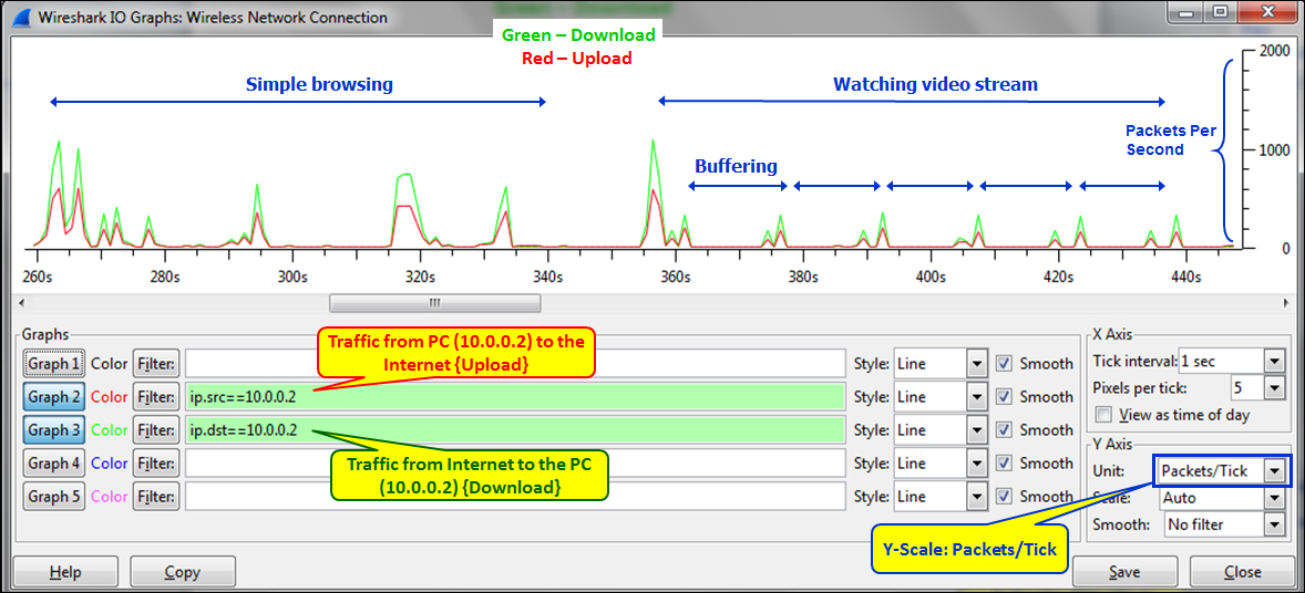
In the first graph, we see that we've measured the traffic when the X Axis is configured to a tick interval of one second and the Y-Axis scale is configured to packets/tick. The result that we've got is that while browsing (on the left-hand side of the graph) or while watching a movie (on the right-hand side of the graph), the upload and download traffic is nearly identical.
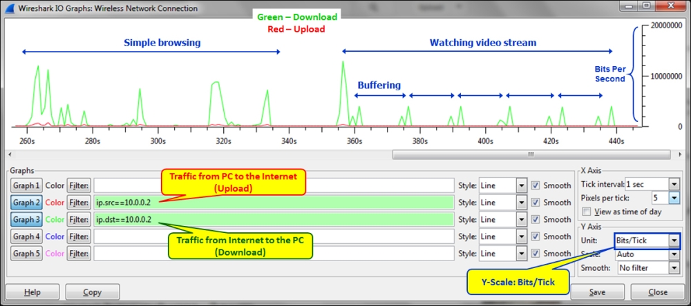
In the second graph, we see the traffic in bits/sec. Here, we see the bandwidth required from the network while using it to connect to the Internet; that is, an asymmetrical bandwidth when most of the traffic is in the download direction.
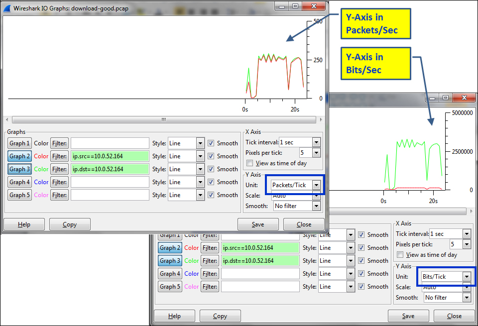
Let's have a look at another example here. This is an example of a file download in FTP when 10.0.52.164 downloads a file. Again, you can see that in order to get the traffic on the network, we changed Unit: under Y-Axis to Bits/Tick. Packets/Tick is also important and we will see implementations for it in the applications chapters (chapters 7-14) later in the book.