
Support Vector Machines (SVMs) are a set of supervised learning techniques for classification and regression (and also for outlier detection), which is quite versatile as it can fit both linear and nonlinear models thanks to the availability of special functions—kernel functions. The specialty of such kernel functions is to be able to map the input features into a new, more complex feature vector using a limited amount of computations. Kernel functions nonlinearly recombine the original features, making possible the mapping of the response by very complex functions. In such a sense, SVMs are comparable to neural networks as universal approximators, and thus can boast a similar predictive power in many problems.
Contrary to the linear models seen in the previous chapter, SVMs started as a method to solve classification problems, not regression ones.
SVMs were invented at the AT&T laboratories in the '90s by the mathematician, Vladimir Vapnik, and computer scientist, Corinna Cortes (but there are also many other contributors that worked with Vapnik on the algorithm). In essence, an SVM strives to solve a classification problem by finding a particular hyperplane separating the classes in the feature space. Such a particular hyperplane has to be characterized as being the one with the largest separating margin between the boundaries of the classes (the margin is to be intended as the gap, the space between the classes themselves, empty of any example).
Such intuition implies two consequences:
- Empirically, SVMs try to minimize the test error by finding a solution in the training set that is exactly in the middle of the observed classes, thus the solution is clearly computational (it is an optimization based on quadratic programming—https://en.wikipedia.org/wiki/Quadratic_programming).
- As the solution is based on just the boundaries of the classes as set by the adjoining examples (called the support vectors), the other examples can be ignored, making the technique insensible to outliers and less memory-intensive than methods based on matrix inversion such as linear models.
Given such a general overview on the algorithm, we will be spending a few pages pointing out the key formulations that characterize SVMs. Although a complete and detailed explanation of the method is beyond the scope of this book, sketching how it works can indeed help figure out what is happening under the hood of the technique and provide the foundation to understand how it can be made scalable to big data.
Historically, SVMs were thought as hard-margin classifiers, just like the perceptron. In fact, SVMs were initially set trying to find two hyperplanes separating the classes whose reciprocal distance was the maximum possible. Such an approach worked perfectly with linearly-separable synthetic data. Anyway, in the hard-margin version, when an SVM faced nonlinearly separable data, it could only succeed using nonlinear transformations of the features. However, they were always deemed to fail when misclassification errors were due to noise in data instead of non-linearity.
For such a reason, softmargins were introduced by means of a cost function that took into account how serious the error was (as hard margins kept track only if an error occurred), thus allowing a certain tolerance to misclassified cases whose error was not too big because they were placed next to the separating hyperplane.
Since the introduction of softmargins, SVMs also became able to withstand non-separability caused by noise. Softmargins were simply introduced by building the cost function around a slack variable that approximates the number of misclassified examples. Such a slack variable is also called the empirical risk (the risk of making a wrong classification as seen from the training data point of view).
In mathematical formulations, given a matrix dataset X of n examples and m features and a response vector expressing the belonging to a class in terms of +1 (belonging) and -1 (not belonging), a binary classification SVM strives to minimize the following cost function:
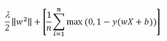
In the preceding function, w is the vector of coefficients that expresses the separating hyperplane together with the bias b, representing the offset from the origin. There is also lambda (λ>=0), which is the regularization parameter.
For a better understanding of how the cost function works, it is necessary to divide it into two parts. The first part is the regularization term:

The regularization term is contrasting the minimization process when the vector w assumes high values. The second term is called the loss term or slack variable, and actually is the core of the SVM minimization procedure:
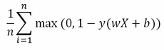
The loss term outputs an approximate value of misclassification errors. In fact, the summation will tend to add a unit value for each classification error, whose total divided by n, the number of examples, will provide an approximate proportion of the classification error.
Often, as in the Scikit-learn implementation, the lambda is removed from the regularization term and replaced by a misclassification parameter C multiplying the loss term:
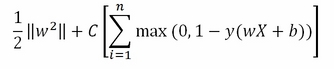
The relation between the previous parameter lambda and the new C is as follows:

It is just a matter of conventions, as the change from the parameter lambda to C on the optimization's formula doesn't imply different results.
The impact of the loss term is mediated by a hyperparameter C. High values of C impose a high penalization on errors, thus forcing the SVM to try to correctly classify all the training examples. Consequently, larger C values tend to force the margin to be tighter and take into consideration fewer support vectors. Such a reduction of the margin translates into an increased bias and reduced variance.
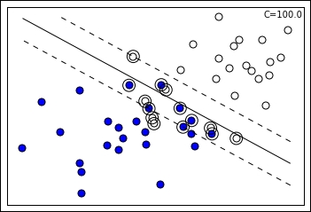
This leads us to specify the role of certain observations with respect to others; in fact, we define as support vectors those examples that are misclassified or not classified with confidence as they are inside the margin (noisy observations that make class separation impossible). Optimization is possible taking into account only such examples, making SVM a memory-efficient technique indeed:
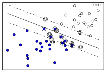
In the preceding visualization, you can notice the projection of two groups of points (blue and white) on two feature dimensions. An SVM solution with the C hyperparameter set to 1.0 can easily discover a separating line (in the plot represented as the continuous line), though there are some misclassified cases on both sides. In addition, the margin can be visualized (defined by the two dashed lines), being identifiable thanks to the support vectors of the respective class further from the separating line. In the chart, support vectors are marked by an external circle and you can actually notice that some support vectors are outside the margin; this is because they are misclassified cases and the SVM has to keep track of them for optimization purposes as their error is considered in the loss term:
Increasing the C value, the margin tends to restrict as the SVM is taking into account fewer support vectors in the optimization process. Consequently, the slope of the separating line also changes.
On the contrary, smaller C values tend to relax the margin, thus increasing the variance. Extremely small C values can even lead the SVM to consider all the example points inside the margin. Smaller C values are ideal when there are many noisy examples. Such a setting forces the SVM to ignore many misclassified examples in the definition of the margin (Errors are weighted less, so they are tolerated more when searching for the maximum margin.):
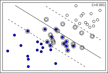
Continuing on the previous visual example, if we decrease the hyperparameter C, the margin actually expands because the number of the support vectors increases. Consequently, the margin being different, SVM resolves for a different separating line. There is no C value that can be deemed correct before being tested on data; the right value always has to be empirically found by cross-validation. By far, C is considered the most important hyperparameter in an SVM, to be set after deciding what kernel function to use.
Kernel functions instead map the original features into a higher-dimensional space by combining them in a nonlinear way. In such a way, apparently non-separable groups in the original feature space may turn separable in a higher-dimensional representation. Such a projection doesn't need too complex computations in spite of the fact that the process of explicitly transforming the original feature values into new ones can generate a potential explosion in the number of the features when projecting to high dimensionalities. Instead of doing such cumbersome computations, kernel functions can be simply plugged into the decision function, thus replacing the original dot product between the features and coefficient vector and obtaining the same optimization result as the explicit mapping would have had. (Such plugging is called the kernel trick because it is really a mathematical trick.)
Standard kernel functions are linear functions (implying no transformations), polynomial functions, radial basis functions (RBF), and sigmoid functions. To provide an idea, the RBF function can be expressed as follows:
Basically, RBF and the other kernels just plug themselves directly into a variant of the previously seen function to be minimized. The previously seen optimization function is called the primal formulation whereas the analogous re-expression is called the dual formulation:

Though passing from the primal to the dual formulation is quite challenging without a mathematical demonstration, it is important to grasp that the kernel trick, given a kernel function that compares the examples by couples, is just a matter of a limited number of calculations with respect to the infinite dimensional feature space that it can unfold. Such a kernel trick renders the algorithm so particularly effective (comparable to neural networks) with respect to quite complex problems such as image recognition or textual classification:
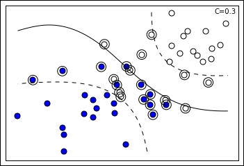
For instance, the preceding SVM solution is possible thanks to a sigmoid kernel, whereas the following one is due to an RBF one:
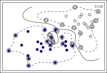
As visually noticeable, the RBF kernel allows quite complex definitions of the margin, even splitting it into multiple parts (and an enclave is noticeable in the preceding example).
The formulation of the RBF kernel is as follows:
Gamma is a hyperparameter for you to define a-priori. The kernel transformation creates some sort of classification bubbles around the support vectors, thus allowing the definition of very complex boundary shapes by merging the bubbles themselves.
The formulation of the sigmoid kernel is as follows:
Here, apart from gamma, r should be also chosen for the best result.
Clearly, solutions based on sigmoid, RBF, and polynomial, (Yes, it implicitly does the polynomial expansion that we will talk about in the following paragraphs.) kernels present more variance than the bias of the estimates, thus requiring a severe validation when deciding their adoption. Though an SVM is resistant to overfitting, it is not certainly immune to it.
Support vector regression is related to support vector classification. It varies just for the notation (more similar to a linear regression, using betas instead of a vector w of coefficients) and loss function:
Noticeably, the only significant difference is the loss function L-epsilon, which is insensitive to errors (thus not computing them) if examples are within a certain distance epsilon from the regression hyperplane. The minimization of such a cost function optimizes the result for a regression problem, outputting values and not classes.
As concluding remarks about the inner nuts and bolts of an SVM, remember that the cost function at the core of the algorithm is the hinge loss:
As seen before, ŷ is expressed as the summation of the dot product of X and coefficient vector w with the bias b:
Reminiscent of the perceptron, such a loss function penalizes errors linearly, expressing an error when the example is classified on the wrong side of the margin, proportional to its distance from the margin itself. Though convex, having the disadvantage of not being differentiable everywhere, it is sometimes replaced by always differentiable variants such as the squared hinge loss (also called L2 loss whereas L1 loss is the hinge loss):
Another variant is the Huber loss, which is a quadratic function when the error is equal or below a certain threshold value h but a linear function otherwise. Such an approach mixes L1 and L2 variants of the hinge loss based on the error and it is an alternative quite resistant to outliers as larger error values are not squared, thus requiring fewer adjustments by the learning SVM. Huber loss is also an alternative to log loss (linear models) because it is faster to calculate and able to provide estimates of class probabilities (the hinge loss does not have such a capability).
From a practical point of view, there are no particular reports that Huber loss or L2 hinge loss can consistently perform better than hinge loss. In the end, the choice of a cost function just boils down to testing the available functions with respect to every different learning problem. (According to the principle of the no-free-lunch theorem, in machine learning, there are no solutions suitable for all the problems.)
Scikit-learn offers an implementation of SVM using two C++ libraries (with a C API to interface with other languages) developed at the National Taiwan University, A Library for Support Vector Machines (LIBSVM) for SVM classification and regression (http://www.csie.ntu.edu.tw/~cjlin/libsvm/) and LIBLINEAR for classification problems using linear methods on large and sparse datasets (http://www.csie.ntu.edu.tw/~cjlin/liblinear/). Having both the libraries free to use, quite fast in computations, and already tested in quite a number of other solutions, all Scikit-learn implementations in the sklearn.svm module rely on one or the other, (The Perceptron and LogisticRegression classes also make use of them, by the way.) making Python just a convenient wrapper.
On the other hand, SGDClassifier and SGDRegressor use a different implementation as neither LIBSVM nor LIBLINEAR have an online implementation, both being batch learning tools. In fact, when operating, both LIBSVM and LIBLINEAR perform the best when allocated a suitable memory for kernel operations via the cache_size parameter.
The implementations for classification are as follows:
|
Class |
Purpose |
Hyperparameters |
|---|---|---|
|
|
The LIBSVM implementation for binary and multiclass linear and kernel classification |
C, kernel, degree, gamma |
|
|
same as above |
nu, kernel, degree, gamma |
|
|
Unsupervised detection of outliers |
nu, kernel, degree, gamma |
|
|
Based on LIBLINEAR, it is a binary and multiclass linear classifier |
Penalty, loss, C |
As for regression, the solutions are as follows:
|
Class |
Purpose |
Hyperparameters |
|---|---|---|
|
|
The LIBSVM implementation for regression |
C, kernel, degree, gamma, epsilon |
|
|
same as above |
nu, C, kernel, degree, gamma |
As you can see, there are quite a few hyperparameters to be tuned for each version, making SVMs good learners when using default parameters and excellent ones when properly tuned by cross-validation, using GridSearchCV from the grid_search module in Scikit-learn.
As a golden rule, some parameters influence the result more and so should be fixed beforehand, others being dependent on their values. According to such an empirical rule, you have to correctly set the following parameters (ordered by rank of importance):
C: This is the penalty value that we discussed before. Decreasing it makes the margin larger, thus ignoring more noise but also making for more computations. A best value can be normally looked for in thenp.logspace(-3, 3, 7)range.kernel: This is the non-linearity workhorse because an SVM can be set tolinear,poly,rbf,sigmoid, or a custom kernel (for experts!). The widely used one is certainlyrbf.degree: This works withkernel='poly', signaling the dimensionality of the polynomial expansion. It is ignored by other kernels. Usually, values from 2-5 work the best.gamma: This is a coefficient for'rbf','poly', and'sigmoid'; high values tend to fit data in a better way. The suggested grid search range isnp.logspace(-3, 3, 7).nu: This is for regression and classification withnuSVRandnuSVC; this parameter approximates the training points that are not classified with confidence, misclassified points, and correct points inside or on the margin. It should be a number in the range [0,1] as it is a proportion relative to your training set. In the end, it acts as C with high proportions enlarging the margin.epsilon: This parameter specifies how much error an SVR is going to accept by defining an epsilon large range where no penalty is associated with respect to the true value of the point. The suggested search range isnp.insert(np.logspace(-4, 2, 7),0,[0]).penalty,lossanddual: For LinearSVC, these parameters accept the('l1','squared_hinge',False),('l2','hinge',True),('l2','squared_hinge',True), and('l2','squared_hinge',False)combinations. The('l2','hinge',True)combination is equivalent to theSVC(kernel='linear')learner.
As an example for basic classification and regression using SVC and SVR from Scikit-learn's sklearn.svm module, we will work with the Iris and Boston datasets, a couple of popular toy datasets (http://scikit-learn.org/stable/datasets/).
First, we will load the Iris dataset:
In: from sklearn import datasets
iris = datasets.load_iris()
X_i, y_i = iris.data, iris.target
Then, we will fit an SVC with an RBF kernel (C and gamma were chosen on the basis of other known examples in Scikit-learn) and test the results using the cross_val_score function:
from sklearn.svm import SVC
from sklearn.cross_validation import cross_val_score
import numpy as np
h_class = SVC(kernel='rbf', C=1.0, gamma=0.7, random_state=101)
scores = cross_val_score(h_class, X_i, y_i, cv=20, scoring='accuracy')
print 'Accuracy: %0.3f' % np.mean(scores)

Output: Accuracy: 0.969
The fitted model can provide you with an index pointing out what are the support vectors among your training examples:
In: h_class.fit(X_i,y_i)
print h_class.support_

Out: [ 13  14  15  22  24  41  44  50  52  56  60  62  63  66  68  70  72  76  77  83  84  85  98 100 106 110 114 117 118 119 121 123 126 127 129 131 133 134 138 141 146 149]
Here is a graphical representation of the support vectors selected by the SVC for the Iris dataset, represented with color decision boundaries (we tested a discrete grid of values in order to be able to project for each area of the chart what class the model will predict):

Tip
If you are interested in replicating the same charts, you can have a look and tweak this code snippet from http://scikit-learn.org/stable/auto_examples/svm/plot_iris.html.
To test an SVM regressor, we decided to try SVR with the Boston dataset. First, we upload the dataset in the core memory and then we randomize the ordering of examples as, noticeably, such a dataset is actually ordered in a subtle fashion, thus making results from not order-randomized cross-validation invalid:
In: import numpy as np
from sklearn.datasets import load_boston
from sklearn.preprocessing import StandardScaler
scaler = StandardScaler()
boston = load_boston()
shuffled = np.random.permutation(boston.target.size)
X_b = scaler.fit_transform(boston.data[shuffled,:])
y_b = boston.target[shuffled]
Tip
Due to the fact that we used the permutation function from the random module in the NumPy package, you may obtain a differently shuffled dataset and consequently a slightly different cross-validated score from the following test. Moreover, the features having different scales, it is a good practice to standardize the features so that they will have zero-centered mean and unit variance. Especially when using SVM with kernels, standardization is indeed crucial.
Finally, we can fit the SVR model (we decided on some C, gamma, and epsilon parameters that we know work fine) and, using cross-validation, we evaluate it by the root mean squared error:
In: from sklearn.svm import SVR
from sklearn.cross_validation import cross_val_score
h_regr = SVR(kernel='rbf', C=20.0, gamma=0.001, epsilon=1.0)
scores = cross_val_score(h_regr, X_b, y_b, cv=20, scoring='mean_squared_error')
print 'Mean Squared Error: %0.3f' % abs(np.mean(scores))

Out: Mean Squared Error: 28.087
SVMs have quite a few advantages over other machine learning algorithms:
- They can handle majority of the supervised problems such as regression, classification, and anomaly detection, though they are actually best at binary classification.
- They provide a good handling of noisy data and outliers and they tend to overfit less as they only work with support vectors.
- They work fine with wide datasets (more features than examples); though, as with other machine learning algorithms, an SVM would gain both from dimensionality reduction and feature selection.
As drawbacks, we have to mention the following:
- They provide just estimates, but no probabilities unless you run some time-consuming and computationally-intensive probability calibration by means of Platt scaling
- They scale super-linearly with the number of examples
In particular, the last drawback puts a strong limitation on the usage of SVMs for large datasets. The optimization algorithm at the core of this learning technique—quadratic programming—scales in the Scikit-learn implementation between O(number of feature * number of samples^2) and O(number of feature * number of samples^3), a complexity that seriously limits the operability of the algorithm to datasets that are under 10^4 number of cases.
Again, as seen in the last chapter, there are just a few options when you give a batch algorithm and too much data: subsampling, parallelization, and out-of-core learning by streaming. Subsampling and parallelization are seldom quoted as the best solutions, streaming being the favored approach to implement SVMs with large-scale problems.
However, though less used, subsampling is quite easy to implement leveraging reservoir sampling, which can produce random samples rapidly from streams derived from datasets and infinite online streams. By subsampling, you can produce multiple SVM models, whose results can be averaged for better results. The predictions from multiple SVM models can even be stacked, thus creating a new dataset, and used to build a new model fusing the predictive capabilities of all, which will be described in Chapter 6, Classification and Regression Trees at Scale.
Reservoir sampling is an algorithm for randomly choosing a sample from a stream without having prior knowledge of how long the stream is. In fact, every observation in the stream has the same probability of being chosen. Initialized with a sample taken from the first observations in the stream, each element in the sample can be replaced at any moment by the example in the stream according to a probability proportional to the number of elements streamed up so far. So, for instance, when the i-th element of the stream arrives, it has a probability of being inserted in place of a random element in the sample. Such an insertion probability is equivalent to the sample dimension divided by i; therefore, it is progressively decreasing with respect to the stream length. If the stream is infinite, stopping at any time assures that the sample is representative of the elements seen so far.
In our example, we draw two random, mutually exclusive samples from the stream—one to train and one to test. We will extract such samples from the Covertype database, using the original ordered file. (As we will stream all the data before taking the sample, the random sampling won't be affected by the ordering.) We decided on a training sample of 5,000 examples, a number that should scale well on most desktop computers. As for the test set, we will be using 20,000 examples:
In: from random import seed, randint
SAMPLE_COUNT = 5000
TEST_COUNT   = 20000
seed(0) # allows repeatable results
sample = list()
test_sample = list()
for index, line in enumerate(open('covtype.data','rb')):
    if index < SAMPLE_COUNT:
        sample.append(line)
    else:
        r = randint(0, index)
        if r < SAMPLE_COUNT:
            sample[r] = line
        else:
            k = randint(0, index)
            if k < TEST_COUNT:
                if len(test_sample) < TEST_COUNT:
                    test_sample.append(line)
                else:
                    test_sample[k] = line
The algorithm should be streaming quite fast on the over 500,000 rows of the data matrix. In fact, we really did no preprocessing during the streaming in order to keep it the fastest possible. We consequently now need to transform the data into a NumPy array and standardize the features:
In: import numpy as np
from sklearn.preprocessing import StandardScaler
for n,line in enumerate(sample):
        sample[n] = map(float,line.strip().split(','))
y = np.array(sample)[:,-1]
scaling = StandardScaler()
X = scaling.fit_transform(np.array(sample)[:,:-1])
Once done with the training data X, y, we have to process the test data in the same way; particularly, we will have to standardize the features using standardization parameters (means and standard deviations) as in the training sample:
In: for n,line in enumerate(test_sample):
        test_sample[n] = map(float,line.strip().split(','))
yt = np.array(test_sample)[:,-1]
Xt = scaling.transform(np.array(test_sample)[:,:-1])
When both train and test sets are ready, we can fit the SVC model and predict the results:
In: from sklearn.svm import SVC
h = SVC(kernel='rbf', C=250.0, gamma=0.0025, random_state=101)
h.fit(X,y)
prediction = h.predict(Xt)
from sklearn.metrics import accuracy_score
print accuracy_score(yt, prediction)

Out: 0.75205
Given the limitations of subsampling (first of all, the underfitting with respect to models trained on larger datasets), the only available option when using Scikit-learn for linear SVMs applied to large-scale streams remains the SGDClassifier and SGDRegressor methods, both available in the linear_model module. Let's see how to use them at their best and improve our results on the example datasets.
We are going to leverage the previous examples seen in the chapter for linear and logistic regression and transform them into an efficient SVM. As for classification, it is required that you set the loss type using the loss hyperparameter. The possible values for the parameter are 'hinge', 'squared_hinge', and 'modified_huber'. All such loss functions were previously introduced and discussed in this same chapter when dealing with the SVM formulation.
All of them imply applying a soft-margin linear SVM (no kernels), thus resulting in an SVM resistant to misclassifications and noisy data. However, you may also try to use the loss 'perceptron', a type of loss that results in a hinge loss without margin, a solution suitable when it is necessary to resort to a model with more bias than the other possible loss choices.
Two aspects have to be taken into account to gain the best results when using such a range of hinge loss functions:
- When using any loss function, the stochastic gradient descent turns lazy, updating the vector of coefficients only when an example violates the previously defined margins. This is quite contrary to the loss function in the log or squared error, when actually every example is considered for the update of the coefficients' vector. In case there are many features involved in the learning, such a lazy approach leads to a resulting sparser vector of coefficients, thus reducing the overfitting. (A denser vector implies more overfitting because some coefficients are likely to catch more noise than signals from the data.)
- Only the
'modified_huber'loss allows probability estimation, making it a viable alternative to the log loss (as found in the stochastic logistic regression). A modified Huber is also a better performer when dealing with multiclass one-vs-all (OVA) predictions as the probability outputs of the multiple models are better than the standard decision functions characteristic of hinge loss (probabilities work better than the raw output of the decision functions as they are on the same scale, bounded from 0 to 1). This loss function works by deriving a probability estimate directly from the decision function:(clip(decision_function(X), -1, 1) + 1) / 2.
As for regression problems, SGDRegressor offers two SVM loss options:
'epsilon_insensitive'
'squared_epsilon_insensitive'
Both activate a linear support vector regression, where errors (residual from the prediction) within the epsilon value are ignored. Past the epsilon value, the epsilon_insensitive loss considers the error as it is. The squared_epsilon_insensitive loss operates in a similar way though the error here is more penalizing as it is squared, with larger errors influencing the model building more.
In both cases, setting the correct epsilon hyperparameter is critical. As a default value, Scikit-learn suggests epsilon=0.1, but the best value for your problem has to be found by means of grid-search supported by cross-validation, as we will see in the next paragraphs.
Note that among regression losses, there is also a 'huber' loss available that does not activate an SVM kind of optimization but just modifies the usual 'squared_loss' to be insensible to outliers by switching from squared to linear loss past a distance of the value of the epsilon parameter.
As for our examples, we will be repeating the streaming process a certain number of times in order to demonstrate how to set different hyperparameters and transform features; we will use some convenient functions in order to reduce the number of repeated lines of code. Moreover, in order to speed up the execution of the examples, we will put a limit to the number of cases or tolerance values that the algorithm refers to. In such a way, both the training and validation times are kept at a minimum and no example will require you to wait more minutes than the time for a cup of tea or coffee.
As for the convenient wrapper functions, the first one will have the purpose to initially stream part or all the data once (we set a limit using the max_rows parameter). After completing the streaming, the function will be able to figure out all the categorical features' levels and record the different ranges of the numeric features. As a reminder, recording ranges is an important aspect to take care of. Both SGD and SVM are algorithms sensible to different range scales and they perform worse when working with a number outside the [-1,1] range.
As an output, our function will return two trained Scikit-learn objects: DictVectorizer (able to transform feature ranges present in a dictionary into a feature vector) and MinMaxScaler to rescale numeric variables in the [0,1] range (useful to keep values sparse in the dataset, thus keeping memory usage low and achieving fast computations when most values are zero). As a unique constraint, it is necessary for you to know the feature names of the numeric and categorical variables that you want to use for your predictive model. Features not enclosed in the lists' feed to the binary_features or numeric_features parameters actually will be ignored. When the stream has no features' names, it is necessary for you to name them using the fieldnames parameter:
In: import csv, time, os
import numpy as np
from sklearn.linear_model import SGDRegressor
from sklearn.feature_extraction import DictVectorizer
from sklearn.preprocessing import MinMaxScaler
from scipy.sparse import csr_matrix

def explore(target_file, separator=',', fieldnames= None, binary_features=list(), numeric_features=list(), max_rows=20000):
    """
    Generate from an online style stream a DictVectorizer and a MinMaxScaler.

    Parameters
----------
    target file = the file to stream from
    separator = the field separator character
    fieldnames = the fields' labels (can be omitted and read from file)
    binary_features = the list of qualitative features to consider
    numeric_features = the list of numeric futures to consider
    max_rows = the number of rows to be read from the stream (can be None)
    """
    features = dict()
    min_max  = dict()
    vectorizer = DictVectorizer(sparse=False)
    scaler = MinMaxScaler()
    with open(target_file, 'rb') as R:
        iterator = csv.DictReader(R, fieldnames, delimiter=separator)
        for n, row in enumerate(iterator):
            # DATA EXPLORATION
            for k,v in row.iteritems():
                if k in binary_features:
                    if k+'_'+v not in features:
                        features[k+'_'+v]=0
                elif k in numeric_features:
                    v = float(v)
                    if k not in features:
                        features[k]=0
                        min_max[k] = [v,v]
                    else:
                        if v < min_max[k][0]:
                            min_max[k][0]= v
                        elif v > min_max[k][1]:
                            min_max[k][1]= v
                else:
                    pass # ignore the feature
            if max_rows and n > max_rows:
                break
    vectorizer.fit([features])
    A = vectorizer.transform([{f:0 if f not in min_max else min_max[f][0] for f in vectorizer.feature_names_},
{f:1 if f not in min_max else min_max[f][1] for f in vectorizer.feature_names_}])
    scaler.fit(A)
return vectorizer, scalerThe second function will instead just pull out the data from the stream and transform it into a feature vector, normalizing the numeric features if a suitable MinMaxScaler object is provided instead of a None setting:
In: def pull_examples(target_file, vectorizer, binary_features, numeric_features, target, min_max=None, separator=',',
fieldnames=None, sparse=True):
    """
    Reads a online style stream and returns a generator of normalized feature vectors

    Parameters
----------
    target file = the file to stream from
    vectorizer = a DictVectorizer object
    binary_features = the list of qualitative features to consider
    numeric_features = the list of numeric features to consider
    target = the label of the response variable
    min_max = a MinMaxScaler object, can be omitted leaving None
    separator = the field separator character
    fieldnames = the fields' labels (can be omitted and read from file)
    sparse = if a sparse vector is to be returned from the generator
    """
    with open(target_file, 'rb') as R:
        iterator = csv.DictReader(R, fieldnames, delimiter=separator)
        for n, row in enumerate(iterator):
            # DATA PROCESSING
            stream_row = {}
            response = np.array([float(row[target])])
            for k,v in row.iteritems():
                if k in binary_features:
                    stream_row[k+'_'+v]=1.0
                else:
                    if k in numeric_features:
                        stream_row[k]=float(v)
            if min_max:
                features = min_max.transform(vectorizer.transform([stream_row]))
            else:
                features = vectorizer.transform([stream_row])
            if sparse:
                yield(csr_matrix(features), response, n)
            else:
                yield(features, response, n)
Given these two functions, now let's try again to model the first regression problem seen in the previous chapter, the bike-sharing dataset, but using a hinge loss this time instead of the mean squared errors that we used before.
As the first step, we provide the name of the file to stream and a list of qualitative and numeric variables (as derived from the header of the file and initial exploration of the file). The code of our wrapper function will return some information on the hot-coded variables and value ranges. In this case, most of the variables will be binary ones, a perfect situation for a sparse representation, as most values in our dataset are plain zero:
In: source = '\bikesharing\hour.csv'
local_path = os.getcwd()
b_vars = ['holiday','hr','mnth', 'season','weathersit','weekday','workingday','yr']
n_vars = ['hum', 'temp', 'atemp', 'windspeed']
std_row, min_max = explore(target_file=local_path+''+source, binary_features=b_vars, numeric_features=n_vars)
print 'Features: '
for f,mv,mx in zip(std_row.feature_names_, min_max.data_min_, min_max.data_max_):
    print '%s:[%0.2f,%0.2f] ' % (f,mv,mx)

Out:
Features:
atemp:[0.00,1.00]
holiday_0:[0.00,1.00]
holiday_1:[0.00,1.00]
...
workingday_1:[0.00,1.00]
yr_0:[0.00,1.00]
yr_1:[0.00,1.00]
As you can notice from the output, qualitative variables have been encoded using their variable name and adding, after an underscore character, their value and transformed into binary features (which has the value of one when the feature is present, otherwise it is set to zero). Note that we are always using our SGD models with the average=True parameter in order to assure a faster convergence (this corresponds to using the
Averaged Stochastic Gradient Descent (ASGD) model as discussed in the previous chapter.):
In:from sklearn.linear_model import SGDRegressor
SGD = SGDRegressor(loss='epsilon_insensitive', epsilon=0.001, penalty=None, random_state=1, average=True)
val_rmse = 0
val_rmsle = 0
predictions_start = 16000

def apply_log(x): return np.log(x + 1.0)
def apply_exp(x): return np.exp(x) - 1.0

for x,y,n in pull_examples(target_file=local_path+''+source,
                           vectorizer=std_row, min_max=min_max,
                           binary_features=b_vars, numeric_features=n_vars, target='cnt'):
    y_log = apply_log(y)
# MACHINE LEARNING
    if (n+1) >= predictions_start:
        # HOLDOUT AFTER N PHASE
        predicted = SGD.predict(x)
        val_rmse += (apply_exp(predicted) - y)**2
        val_rmsle += (predicted - y_log)**2
        if (n-predictions_start+1) % 250 == 0 and (n+1) > predictions_start:
            print n,
            print '%s holdout RMSE: %0.3f' % (time.strftime('%X'), (val_rmse / float(n-predictions_start+1))**0.5),
            print 'holdout RMSLE: %0.3f' % ((val_rmsle / float(n-predictions_start+1))**0.5)
    else:
        # LEARNING PHASE
        SGD.partial_fit(x, y_log)
print '%s FINAL holdout RMSE: %0.3f' % (time.strftime('%X'), (val_rmse / float(n-predictions_start+1))**0.5)
print '%s FINAL holdout RMSLE: %0.3f' % (time.strftime('%X'), (val_rmsle / float(n-predictions_start+1))**0.5)

Out:
16249 07:49:09 holdout RMSE: 276.768 holdout RMSLE: 1.801
16499 07:49:09 holdout RMSE: 250.549 holdout RMSLE: 1.709
16749 07:49:09 holdout RMSE: 250.720 holdout RMSLE: 1.696
16999 07:49:09 holdout RMSE: 249.661 holdout RMSLE: 1.705
17249 07:49:09 holdout RMSE: 234.958 holdout RMSLE: 1.642
07:49:09 FINAL holdout RMSE: 224.513
07:49:09 FINAL holdout RMSLE: 1.596
We are now going to try the classification problem of forest covertype:
In: source = 'shuffled_covtype.data'
local_path = os.getcwd()
n_vars = ['var_'+'0'*int(j<10)+str(j) for j in range(54)]
std_row, min_max = explore(target_file=local_path+''+source, binary_features=list(),
                  fieldnames= n_vars+['covertype'], numeric_features=n_vars, max_rows=50000)
print 'Features: '
for f,mv,mx in zip(std_row.feature_names_, min_max.data_min_, min_max.data_max_):
    print '%s:[%0.2f,%0.2f] ' % (f,mv,mx)

Out:
Features:
var_00:[1871.00,3853.00]
var_01:[0.00,360.00]
var_02:[0.00,61.00]
var_03:[0.00,1397.00]
var_04:[-164.00,588.00]
var_05:[0.00,7116.00]
var_06:[58.00,254.00]
var_07:[0.00,254.00]
var_08:[0.00,254.00]
var_09:[0.00,7168.00]
...
After having sampled from the stream and fitted our DictVectorizer and MinMaxScaler objects, we can start our learning process using a progressive validation this time (the error measure is given by testing the model on the cases before they are used for the training), given the large number of examples available. Every certain number of examples as set by the sample variable in the code, the script reports the situation with average accuracy from the most recent examples:
In: from sklearn.linear_model import SGDClassifier
SGD = SGDClassifier(loss='hinge', penalty=None, random_state=1, average=True)
accuracy = 0
accuracy_record = list()
predictions_start = 50
sample = 5000
early_stop = 50000
for x,y,n in pull_examples(target_file=local_path+''+source,
                           vectorizer=std_row,
                           min_max=min_max,
                           binary_features=list(), numeric_features=n_vars,
                           fieldnames= n_vars+['covertype'], target='covertype'):
    # LEARNING PHASE
    if n > predictions_start:
        accuracy += int(int(SGD.predict(x))==y[0])
        if n % sample == 0:
            accuracy_record.append(accuracy / float(sample))
            print '%s Progressive accuracy at example %i: %0.3f' % (time.strftime('%X'), n, np.mean(accuracy_record[-sample:]))
            accuracy = 0
    if early_stop and n >= early_stop:
            break
    SGD.partial_fit(x, y, classes=range(1,8))

Out: ...
19:23:49 Progressive accuracy at example 50000: 0.699
Tip
Having to process over 575,000 examples, we set an early stop to the learning process after 50,000. You are free to modify such parameters according to the power of your computer and time availability. Be warned that the code may take some time. We experienced about 30 minutes of computing on an Intel Core i3 processor clocking at 2.20 GHz.