The Splunk iplocation command is a powerful command that extracts location information such as city, country, continent, latitude, longitude, region, zip code, time zone, and so on from the IP address. This command can be used to extract relevant geographic and location information, and those extracted fields can be used to filter and, create statistical analytics based on location information. Let's suppose we have data with IP addresses of users making transactions on the website. Using the iplocation command, we can find the exact location and analytics, such as the highest number of transactions done from which state or continent, or in a location an e-commerce site is more popular. Such kind of location-based insight can be derived using the iplocation command.

The syntax for the iplocation command is as follows:

… | iplocation
    allfields= True / False 
    prefix=Prefix_String
    IPAddress_fieldname

The description of the parameters of the preceding query is as follows:

Take a look at the following example:

index="web_server" | iplocationallfields=true prefix=VisitorIP_ device_ip | fields + VisitorIP_* device_ip

The output of the preceding query would look similar to the following screenshot:

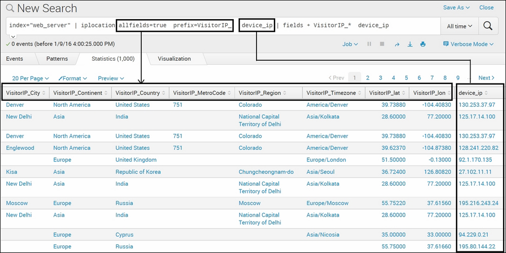
In the preceding example, the allfields parameter is set to true. Hence, all the fields are generated with the respective IP address. Also, the prefix is set to VisitorIP_, and hence, all the fields city, country, continents, and so on are prefixed with the given prefix and the field names are VisitorIP_city, VisitorIP_country, and so on. The IPAddress_fieldname for the preceding example is device_ip, which, as shown in the preceding image is the file with the IP address. Also, in the example, the fields command, which was explained in the previous chapter, is used to display on selected fields, that is, fields that have VisitorIP_ as a prefix and device_ip. In the preceding screenshot, it can be seen that some fields are not populated for some specific IP addresses. This is because the information is fetched from a database, and it may be that not all information is available for respective IP addresses in the database.

The Splunk geostats command is used to create statistical clustering of locations that can be plotted on the geographical world map. If the data on Splunk has an IP address, we can use the iplocation command to get the respective location information. If the data already has location information, then using geostats, the location can be summarized in a way so that it can be plotted on the map. This command is helpful in creating visualization showing the required information on the map marked at its location. Let's suppose, in our web server data, we can use the geostats command to see the count of users doing transactions from all over the world on the map.

The syntax for the geostats command is as follows:

… | geostats
    latfield= Latitude_FieldName
    longfield= Longitude_FieldName
    outputlatfield=Output_Latitude_FieldName
    outputlongfield=Output_Longitude_FieldName
    binspanlat=Bin_Span_Latitude
    binspanlong=Bin_Span_Longitude
    Stats_Agg_Function... by-clause

The parameter description of the geostats command is as follows:

Take a look at the following example:

index="web_server" | iplocationallfields=true prefix=VisitorIP_ device_ip |geostatslatfield=VisitorIP_latlongfield=VisitorIP_lon count by status

The output of the preceding query would look similar to the following screenshot:

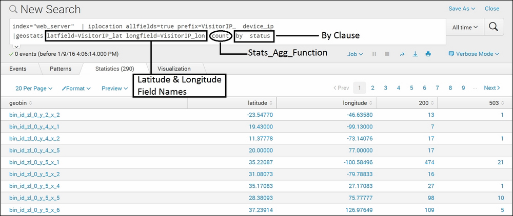
As shown in the preceding example, by running the geostats command, the geobin field with clusters of latitude and longitude are created. They output the information on the world map. Depending on the data and parameters specified, clusters are created accordingly, and hence, the relevant information that is available in the preceding screenshot as a tabular format can be available in the visualization of the world map. You will learn how to create customized world map visualizations in detail in the upcoming chapters.