The Splunk predict command can predict the future values of time series data. Time series is a set of values in the given dataset over time intervals. Examples of time series data can be data generated by machines as per their daily usage. This can be stock values of any script over the day, week, month, year, and so on. Basically, time series data can be any data that has data points over the time interval. Let's take an example. The Predict command can be used to predict the network condition of an LTE network for the next week based on the data of the current month or the number of visitors the website can probably get in the next week, based on the current dataset. Thus, this command can be used to predict future performance, requirements, outages, and so on.

Take a look at the following query block for the syntax:

… | predict
    Fieldname (AS NewFieldName)
    Algorithm = LL / LLP / LLT / LLB / LLP5
    Future_timespan = Timespan
    Period = Period_value
    Correlate = Fieldname

Only the fieldname for which new values are to be predicted is the compulsory parameter. The rest all are optional parameters. The parameter description of the predict command is as follows:

An example query for the predict query is shown as follows:

|inputcsvPrdiction.csv | eval _time=strptime(DateTime, "%d.%m.%Y %H:%M:%S") | timechart span=10m count(Value) AS Value | predict Value as PredictedValue algorithm=LL future_timespan=1

The preceding query should produce an output like the following screenshot:

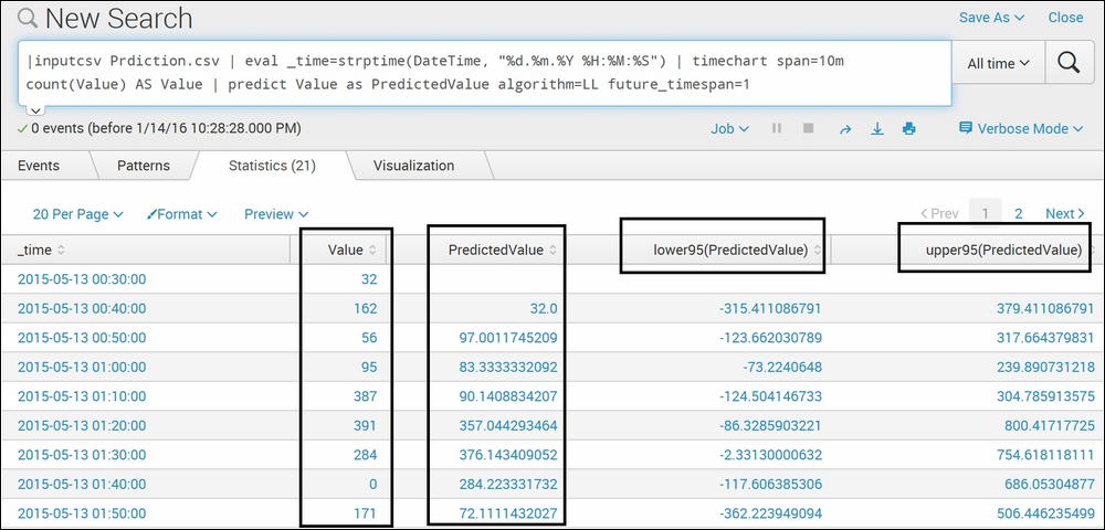
The preceding screenshot shows the tabular (statistical) output of a search result on Splunk web for the predict command. The following screenshot shows the same prediction in the visualization format:

In the preceding screenshot, we used the predict command to predict the next 1 (Future_timespan=1) value of the Value fieldname and the algorithm used is Local Level (LL). We have used the strptime command to format the date and time (field name—DateTime) into Splunk understandable time (field name—_time) format. The predict line chart shows the prediction in a graphical format to understand and visualize the predicted result in a better format. Thus, the predict command can be used to predict the value of the factor specified. The predict command also predicts the lower and upper range of values for the predicted field. This command is very useful in predicting the demand of the product in future, given the historical data, the number of visitors, KPI values, and so on. Thus, it can be used to plan and be ready for future requirements in advance.

The trendline Splunk command is used to generate trends of the dataset for better understanding and visualization of the data. This command can be used to generate moving averages, which includes simple moving average, exponential moving average, and weighted moving average.

The syntax for the trendline command is as follows:

… |trendline (TrendType Period "("Fieldname")" AS NewFieldName)
      TrendType = ema / wma / sma

The description of the parameters of the preceding query is as follows:

Take a look at the following example query:

|inputcsvdatanse.csv | eval _time=strptime (date, "%e-%b-%y") | trendlinesma5(DAX) AS Trend_DAX

The output of the preceding query should look like the following:

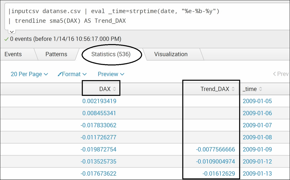
The preceding screenshot shows the statistical output of the trendline command on the Splunk web console, whereas the following screenshot shows the same result in a visualization format:

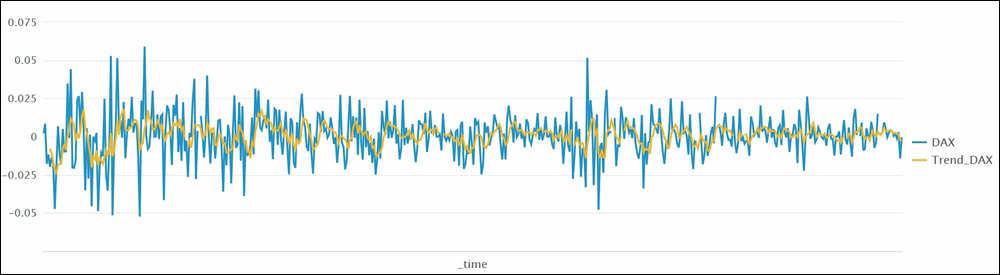
In this example, we used stock index test data. Using the trendline command, the moving average of the DAX field is created as Trend_DAX. The trendline command can calculate different moving averages, such as simple, exponential, and weighted. In this example, we have calculated the simple moving average (sma) with period value as 5, and hence, in the example, you see sma5(DAX). In the visualization, the simple moving average for DAX superimposed with original DAX values can be seen. Thus, the trendline command can be used to calculate and visualize different moving averages of the specified field and proper inference can be made out from the dataset.

The Splunk command x11 is like the trendline command and is also used to create trends for the given time series data. The difference is the method that is based on the x11 algorithm to create the trend. The x11 command can be used to get the real trends of the data by removing seasonal fluctuations in the data.

Take a look at the syntax for the x11 command:

… | x11
    Add() / Mult()
    Period
    Field_name AS New_Field_name

The parameter description for the x11 command is as follows:

Take a look at the following example:

|inputcsvdatanse.csv | eval _time=strptime (date, "%e-%b-%y")| table _time DAX  |x11 DAX AS Trend_X11_DAX

The output generated should be like the one that follows:

The preceding screenshot shows the output of the x11 command in a tabular (statistical) format, whereas the following screenshot shows the same result in the form of visualization:

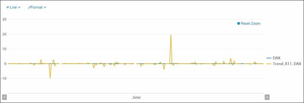
As explained earlier, the Splunk command x11 is used to compute the trends of the data by removing seasonality. The data used to showcase this example is the same as for the trendline command. The output result of both the trendline and x11 commands can be compared as both are commands to compute the trends. The visual difference in the graphs shows how the trends will look like when seasonality is removed while computing the trends.