The correlate Splunk command is used to calculate the correlation between different fields of the events. In simpler terms, it means that this command returns an output that shows what is the co-occurrence between different fields of the given dataset. Let's say I have a dataset that has information about web server failures. Then, using the correlate command, a user can find out whenever there is a failure what other field values have also occurred most of the time. So, insight can be generated to show that whenever X set of events occurs, Y also occurs, and hence, failures can be detected beforehand and action can be taken.

Syntax for the correlate command is as follows:

… | correlate

The example query should looks like the following one:

index="web_server" | correlate

The screenshot that follows shows the output of the preceding query:

This command of Splunk does not require any parameters. The dataset used to showcase this example is a test data, having visitor information on an Apache web server. The correlate Splunk command resulted in a matrix that shows the correlation coefficient of all the fields in the given dataset. The correlation coefficient determines the relation or dependency of the respective fields with each other.

The associate Splunk command is used to identify the correlation between different fields of the given dataset. In general, association in data mining refers to identifying the probability of co-occurrence of items in a collection. The relationship between co-occurring items are expressed as association rules. Similarly, this command identifies the relationship between fields by calculating the change in entropy. According to the Splunk documentation, entropy in this scenario represents whether knowing the value of one field can help in predicting the value of other fields. Association can be explained by the famous bread-butter example. In a supermarket, it is observed that most of the time, when bread is purchased, butter is also purchased, and bread and butter have a strong association.

The syntax for the associate command looks like following:

… | associate 
    Associate-options
    Field-list

The parameter description of the associate command is as follows:

The output of this command will have various fields, namely Reference Key, Value, Target key, Entropy, and Support.

Refer to the following example for better clarity:

index=_internal sourcetype=splunkd | associate

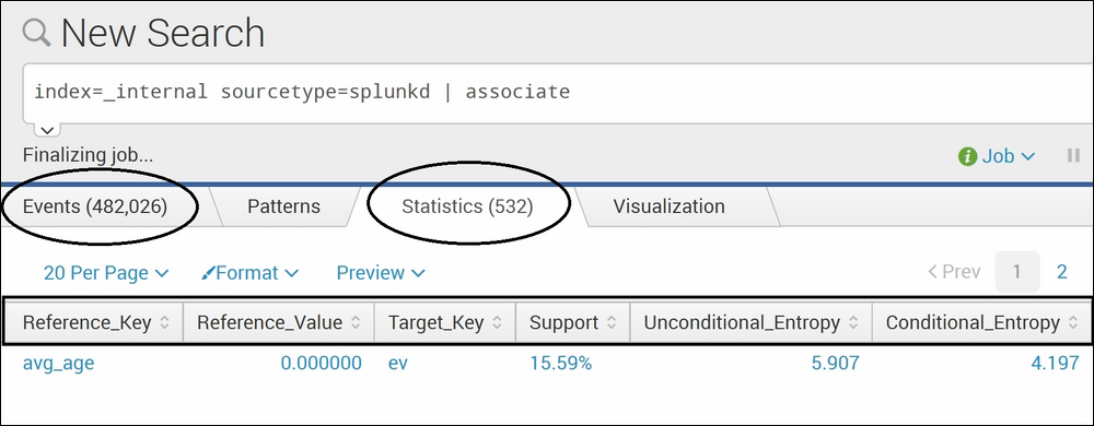
The result of the associate command is quite long horizontally. Hence, the preceding screenshot shows the first section of the result, whereas the following screenshot shows the second section of the result on the Splunk Web console:

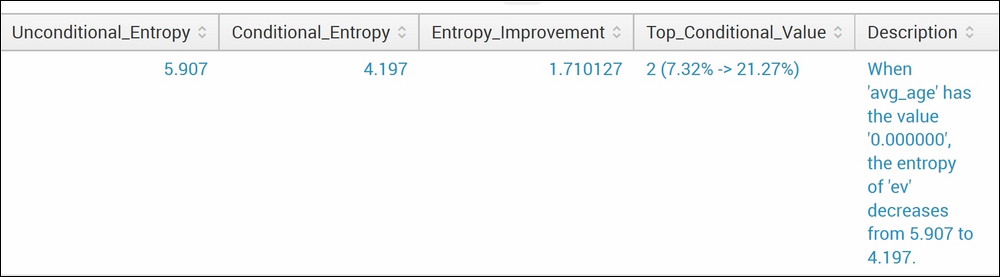
In the preceding example, the associate Splunk command is run on the Splunk internal index (_internal), which logs various activities of the Splunk instance, the sourcetype splunkd logs data that is required to troubleshoot Splunk. The associate command on this data resulted in values in fields such as reference_key, reference_value, target_key, Support, Entropy (Conditional and Unconditional), and Description. As shown in the example, the description parameter explains that when the avg_age has a value of 0.0, the entropy of ev decreases from 5.907 to 4.197. Similarly, the associate command can be run on any data to get the associativity of different fields and various parameters to understand the associativity between them.

The diff Splunk command is used to compare two search results and give line-by-line difference of the same. This command is useful in comparing the data of two similar events and deriving an inference out of it. Let's say we have a failure case due to a Denial of Service (DOS) attack on the web server. Using the diff command, the results of the last few failure cases can be compared, and the difference between those results can be outputted in the result so that such cases can be avoided in future.

The syntax for the diff command looks as follows:

… | diff 
    position1=Position1_no
    position2=Position2_no
    attribute=Field_Name

The parameter description for the diff command is as follows:

Following is an example of the diff command:

index="web_server" | diff position1=19 position2=18

The preceding diff query should produce an output like that in the following screenshot:

The dataset used for this example is the test visitor information of the Apache web server, which was used in earlier examples. The diff Splunk command is used to compare the results of the specified position (in our example, the positions are 19 and 18). The results show that there was no difference between the results of position 18 and 19 for the _raw field as no value was passed to the attribute parameter. Thus, this command can be used to find the difference between the results of two positions.

The contingency Splunk command is used to find support and confidence of the association rule and build a matrix of co-occurrence of values of the given two fields of the dataset. Basically, the contingency table is a matrix that displays the frequency distribution of the variables that can be used to record and analyze the relation between two or more categorical variables. The contingency table can be used to calculate metrics of associations such as the phi coefficient.

Refer to the following query block for the syntax:

… | contingency 
    contingency-options - maxopts / mincover / usetotal / totalstr
    field1
    field2

The description of the parameters of the preceding query is as follows:

Refer to the following example for better clarity:

index="web_server" | contingency useragent device_ip

The following screenshot is the output of the preceding query:

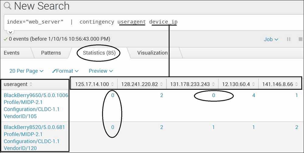
The contingency Splunk command is used build a matrix of co-occurrence of the values. The dataset is the same as the one used in the preceding command example. Here, in this example, the contingency command on fields (useragent and device_ip) resulted in the co-occurrence matrix of both the specified fields. For example, from the first row, inference can be derived that all but the first and third users (device_ip—125.17.14.100 and 131.178.233.243) have accessed the web server from Blackberry9650. Similarly, except the first user (device_ip—125.17.14.100), others have accessed the web server from BlackBerry8520 and so on. Thus, using contingency, such useful hidden insights can be derived and used.