
11
SCALE‐UP OF MASS TRANSFER‐LIMITED REACTIONS: FUNDAMENTALS AND A CASE STUDY
Seth Huggins
Drug Substance Technologies and Engineering, Amgen Inc., Thousand Oaks, CA, USA
Ayman Allian
Synthetic Technologies and Engineering, Amgen Inc., Thousand Oaks, CA, USA
11.1 INTRODUCTION
In the pharmaceutical industry, chemical engineers are challenged to reduce the cost and time to market in drug development; this motivates seamless process scale‐up – that is, translating the process, which has been designed and developed in the lab, to production scale, while maintaining the same process efficiency and product quality. This type of seamless scale‐up, however, is not always easy to achieve and may require a priori understanding of when, and to what extent, an operation might be scale sensitive.
Indeed, unexpected results, such as the formation of new impurities and yield losses, during scale‐up are frequent occurrence. The latter can introduce delays and often require significant resources to rectify. Such scale‐up surprises are not uncommon even when biopharmaceutical companies use their internal pilot plants for scale‐up. To make matters more challenging, in the last decade, low cost manufacturing around the globe particularly in emerging markets like India and China has pushed biopharmaceutical companies to externalize portions, if not all, of their scale‐up operations around the globe. This explosion of outsourcing across pharmaceutical companies has compounded the challenge of scale‐up due to the simple fact that the staff that developed the process in the lab and those in charge of scale‐up are in different geographical locations, with probably different time zones. Consequently, when scale‐up issues do arise in these scenarios, the cost can be even higher, as it often requires development staff to travel and oversee the scale‐up operations in person, resulting in delays and high travel costs. In this current manufacturing paradigm, scientist and staff involved in scale‐up and tech transfer simply cannot afford to fail at scale. This has given rise to heavy emphasis on the concept of right first time [1].
This chapter provides guidance for successful scale‐up of reaction operations: first showing when these operations are likely to be scale sensitive – namely, when there is a strong mass transfer dependence – and then providing a brief review of the fundamentals of mass transfer to illuminate why scale sensitivities exist when mass transfer plays a large role in the overall system dynamics. At the end, an illustrative example of a mass transfer‐limited reaction system is given.
11.1.1 When a Reaction Operation Is Likely Scale Sensitive
The root cause of scale sensitivity is transport phenomena, and not, generally, chemical transformation. Transport phenomena can take a different shape based on the system at hand as outline in the next examples. In processes where gas is required, transport refers to the adsorption of gas to liquid, such as the use of hydrogen to reduce chemical species or oxygen to enable cell growth. For the same system, gas–liquid, there are also operations where inertion of the bulk liquid medium is required to remove undesirable gases such as oxygen and carbon dioxide. For example, removal of oxygen may be required to prevent catalyst/chemistry poisoning. This transport phenomenon commonly referred as gas desorption studies the transport of dissolved gas into bubbles and headspace. In liquid–liquid mixing, transport refers to species transport between micelles or between immiscible phases – as in liquid extraction, a ubiquitous unit operation in pharmaceutical processing. Solid–liquid transport is also very critical to pharmaceutical operations describing the dissolution of suspended solids into solution and is often a dominant mechanism to the startup of a chemical. The transport of dissolved species to solid is the key mechanism in critically important operations like crystallization utilized for the separation and purification of active pharmaceutical ingredients (APIs).
These transport phenomena can be coupled with a reaction, which can complicate understanding the unit operation at hand. For example, in hydrogenation reactions, the hydrogen transport and reaction can take place simultaneously. Solid dissolution can also commonly be coupled with a reaction of the dissolved substance in the bulk liquid. For these various unit operations, the overall observed reaction rate can depend on a number of competing mass transfer and chemical kinetic rate processes that chemical engineers need to understand in order to evaluate these unit operations and how their performance will be impacted by scaling up and/or changing equipment. A common methodology for the assessment of scale sensitivity is carried out by evaluating the rate of mass transfer relative to the rate of chemical transformation using the classical Damköhler number:
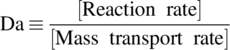
In the case where the Damköhler number is high (e.g. Da > 100), the rate of mass transfer is slow compared with the rate of reaction. The overall observed rate is therefore dictated by the slow rate of mass transfer and very likely to be scale sensitive. On the other hand, when mass transfer is very fast and reaction rate is slower (e.g. Da < 0.01), the overall system dynamics are dictated by the reaction and likely to be scale insensitive. In other words, if the Damköhler number is low, the system dynamics observed at the lab scale are likely to be accurate as the reaction is scaled up, but if Damköhler number is high, scale effects should be anticipated.
11.1.2 Survey of Mass Transfer Challenges in the Pharmaceutical Industry
Understanding mass transfer early on in the process is critical in order to avoid costly delays during scale‐up or tech transfer to pilot plants. Indeed, in a recent survey of 240 cases in which yield or quality was negatively impacted during scale‐up, 30% of these failures were attributed to mass transfer [1]. If we look closer at these cases, Table 11.1, we also see that 50% of those mass transfer challenges are related to solid–liquid systems.
TABLE 11.1 Breakdown of Reported Mass Transfer‐Related Challenges in Scale‐Up
| Systems | Percentage |
| Solid–liquid | 50 |
| Gas–liquid | 20 |
| Liquid–liquid | 20 |
| Solid–gas–liquid | 10 |
The fact that the vast majority of mass transfer challenges are related to solid–liquid systems is not surprising, as most APIs and their intermediates are typically generated in agitated batch reactors that involve solid starting materials, solid reagents, and/or solid catalysts mixed in a liquid solution. If any of the latter species is not completely soluble during the process, i.e. the mixture is heterogeneous, then mass transfer can play a role in overall observed reaction rates with a potential to introduce challenges to scale‐up. While this chapter is focused on solid–liquid mass transfer, the reader should come away with an understanding that is general: mass transfer, and transport phenomena more broadly, depends on the shape, size, and configuration of the reactor and is therefore affected by scale.
11.2 MASS TRANSFER IN A SOLID–LIQUID SYSTEM WITHOUT REACTION
11.2.1 Background
As mentioned earlier, many pharmaceutical unit operations involve a solid phase dispersed in a liquid solution, as shown in Figure 11.1a. For simplicity, we assume the solids are spheres, and agitation is sufficient to ensure particle suspension. Progressively zooming in on the solid–liquid interface, we can highlight the key components that dictate mass transfer. Zooming in one level (Figure 11.1b), we see that the fluid inside the vessel is moving at a certain velocity; however, the fluid velocity directly in contact with the solid sphere is approaching zero due to drag forces. This difference in velocity is referred to as the slip velocity. As we move away from the sphere, drag forces are weakened, and fluid velocity will gradually increase until it reaches the bulk liquid velocity. The distance from the solid surface to the point where the fluid is 99% of the bulk velocity is a critical parameter in solid dissolution and is referred to as the boundary layer thickness, δ [2]. It is generally accepted that all resistance to mass transfer is within the boundary layer. As we will see, the boundary layer thickness is inversely proportional to agitation speed, and, thus, agitation speed can impact mass transfer rate. Zooming in one more level, Figure 11.1c, we illustrate the second key component of mass transfer: a concentration gradient. In our illustration, the solid is assumed to be made up of pure species A, while the solution is a mixture that contains A. In this scenario, the concentration of A is high on the surface of solid (and can generally be assumed to be saturation concentration ![]() ), while the concentration of A is lower in the bulk liquid (at least initially). Consequently, there is a concentration gradient that will drive transport in the direction of decreasing concentration through the boundary layer. Eventually, the concentration in the liquid bulk CA will reach saturation, i.e. solubility limit, and the diffusion will cease.
), while the concentration of A is lower in the bulk liquid (at least initially). Consequently, there is a concentration gradient that will drive transport in the direction of decreasing concentration through the boundary layer. Eventually, the concentration in the liquid bulk CA will reach saturation, i.e. solubility limit, and the diffusion will cease.
FIGURE 11.1 Illustration of transport in a solid‐liquid system showing (a) solid phase, black spheres suspended in a agitated liquid solution, (b) a closer look at a suspended sphere showing the fluid velocity profiles around it and (c) a closer look at the solid-liquid interphase showing the diffusion boundary layer.
Rate of transport in solid–liquid transport is proportional to the concentration gradient and inversely proportional to the boundary layer thickness. Taking the latter parameters, one can calculate the time‐dependent concentration profile of solid‐phase A using the classical chemical engineering equation, also known as the Noyes–Whitney equation, below:
| Rate of mass transfer across the boundary layers |
= | Term 1: kL mass transfer coefficient | Term 2: a interfacial area | Term 3: |
- Term 1 Mass Transfer Coefficient kL: It is worth mentioning that Eq. (11.2) can be derived from Fick's law, which consists the boundary layer thickness δ whose magnitude is unknown. Therefore, and for convenience, mass transfer coefficient is normally used to replace the diffusivity coefficient D and the boundary layer δ as shown in Eq. (11.3):
where D is the solute diffusivity in the bulk liquid in liquid solution across the boundary layer δ. Next, we will assess the dependence of the latter parameters on reactor geometry, i.e. scale‐up. Diffusivity, D, in liquid can be estimated using several approaches like Stokes–Einstein equation or the Wilke–Chang estimates shown in Eq. (11.4):
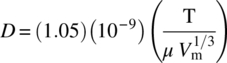
where
- T is temperature in Kelvin.
- μ is the viscosity of the liquid.
- Vm is the molar volume of diffusing species at its boiling point.
The effect of the latter parameters like temperature and viscosity is somewhat expected, i.e. increase in temperature will increase diffusion coefficient and thus the dissolution rate. In addition, increase in solvent viscosity will decrease dissolution rate. The latter parameters are physical properties that are not expected to be scale sensitive. On the other hand, boundary layer thickness δ is a function of velocity profiles within the agitated vessel and therefore very dependent on the reactor geometrical parameters. This includes, but is not limited to, impeller type, size, and speed. Furthermore, baffling and geometry of the system can also impact δ. Changes in these parameters, due to scale or change in equipment, can result in significant changes in δ and thus the overall observed rate that explains the large number of cases where surprises are encountered during scale‐up.
- Term 2 Interfacial Area a: The rate of the mass transfer is directly impacted by the interfacial area per unit volume, a, as shown in Eq. (11.2). An increase in the area will directly increase the overall mass transfer rates. Interfacial area per unit volume of the same solid increases by decreasing particle size that can directly increase the overall mass transfer rate, kLa, assuming kL remains constant.
- Term 3 Concentration Gradient
 : The concentration gradient across the boundary layer, Figure 11.1c, is the driving force for the transport. Typically, the concentration at the surface is high, and diffusion takes place until the concentration in the bulk phase reaches saturation,
  .
.
While the focus has been on solid–liquid mass transfer, the author wants to point out that the dynamics of mass transfer in other multiphase systems follow similar equations. The concepts discussed here can be, in a general sense, extrapolated to other applications such as hydrogenation, gas solubility in a bioreactor, oxygen and CO2 desorption, and even drug dissolution studies in aqueous phase. This is illustrated in Table 11.2, where we show that the mass transfer equations for these different two‐phase systems are either equivalent to, or resemble, Eq. (11.2).
TABLE 11.2 Variation of the Mass Transfer Equation Across Several Transport Systems Discussed in the Current Textbook
| Scenario | Governing Equation | References |
| Gas–liquid H2 mass transfer |
Chapter 9 | |
| Gas–Liquid Oxygen uptake rate in a bioreactor |
Chapter 17 | |
| Gas–Liquid Desorption rate of unwanted gas like O2 and CO2, which can poison the catalyst |
Chapter 8 |
11.2.2 Qualitative Impact of Key Parameter on Mass Transfer Coefficient kL
There are several geometrical parameters that can impact mass transfer coefficient kL and interfacial area a. In this section, more light is shed on the degree of the impact of two key parameters on the overall mass transfer coefficient, kLa, namely, particle size and agitation rate.
11.2.2.1 Effect of Particle Size on the Overall Mass Transfer Coefficient
Particle size has a significant effect on the interfacial area a. In this section we want to highlight the impact of particle size on kL. In contrast to the effect on interfacial area, decreasing the particle size interestingly has a negative effect on kL. However, the effect on kL is very minimal. A study showed that reducing particle size from 10 000 to 40 mm decreased kL by 33% and this reduction is expected to enormously increase the area interfacial area a [3].
11.2.2.2 Agitation Speed and State of Solid Suspension Impact on the Overall Mass Transfer Coefficient
Understating the state of solid suspension in your vessel is very critical to mass transfer. In an agitated vessel, the degree of solid suspension is classified into three states, namely, partial suspension, complete suspension, and uniform suspension, as shown in Figure 11.2 [4]. In the partial suspension, due to no or little stirring, much of the solid is settled at the bottom of reactor. The surface area of the settled particles will not be available, as they are obscured by other particles; therefore, interfacial area in this scenario is low. Once sufficient agitation is reached, we move into State II where solids begin to suspend until complete suspension is realized and no particles remaining at the base of the agitated reactor for more than one to two seconds. At this stage, the entire surface area of the particles is exposed for mass transfer or reaction. The minimum impeller speed required to achieve full suspension is termed the just‐suspended speed and is denoted Njs, as shown Figure 11.2. Uniform suspension occurs when agitation is high enough beyond Njs and at a state where particle size distribution is uniform throughout the agitated vessel (Figure 11.2).
FIGURE 11.2 Mass transfer coefficient over a wide range of stirring speed.
FIGURE 11.3 Mass transfer and reaction in a solid–liquid system.
In the partial suspension (State I), agitation impact is limited to rolling particles at the bottom of the reactor. As we enter into State II, increasing impeller speed has significant positive effect on the relative mass transfer. Specifically, (i) increasing impeller speed will increase the velocity profile in the agitated vessel and consequently decrease the boundary layer thickness, and therefore increase mass transfer, and (ii) increase the portion of the solid particle that are suspended, which will increase the effective interfacial area, and again increase the mass transfer. Indeed, in this region, the overall transfer coefficient kLa will rapidly increase with increasing agitation until reaction complete suspension state. However, increasing impeller speed beyond Njs (State III) improves the homogeneity of the suspension but does not greatly improve the mass transfer characteristics. It is worth noting that increasing agitation speed any further, beyond State III, can bring about surface aeration, NSA, where ingested air due to high agitation blanket the particles surface.
It is clear from the upper discussion that for solid–liquid mass transfer, it is very desirable to operate at an impeller speed ≥Njs, which also means that chemical engineers need to understand and estimate Njs for their vessel wherein scale‐up will take place and ultimately carry out the development in appropriate scale‐down models. In practice, however, this is easier said than done, as the development teams are typically not informed of the site where the process will be scaled until late in development. To estimate Njs, a number of correlations are available. The most widely used correlations for Njs is the Zwietering correlation shown below:
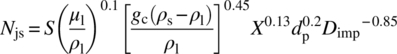
where
- S is a dimensionless number that is a function of the impeller type.
- μl is liquid viscosity.
- ρs is the solid density.
- ρl is bulk liquid density.
- gc is the gravitation constant (9.81 m/s2).
- Dimp is the impeller diameter.
- X is the mass ratio of suspended solids to liquid × 100.
It is critically important to ensure when a heterogeneous reaction is scaled up or to be carried out at a different equipment that particles are well suspended. Typically, scale‐ups are done in stainless steel vessels, visually making sure that solids are suspended can be difficult. However, there are also several tools that can inform us on the state of suspension. Indeed, a recent study showed just monitoring the temperature difference between baffle and bottom of the vessel can be a very effective tool [5].
11.2.3 Measurement and Estimate of Mass Transfer kL for a Solid–Liquid System
Measurement of mass transfer coefficient kL in the pharmaceutical industry is typically done experimentally. In this approach, Eq. (11.2) is integrated with the appropriate boundary conditions. Namely, at time equal zero, the initial concentration of A in the bulk liquid is ![]() , while the concentration at time (t) is CA, and then Eq. (11.2) can be reduced to
, while the concentration at time (t) is CA, and then Eq. (11.2) can be reduced to
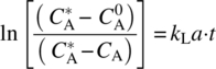
Equation (11.6) resembles a straight line, y = mx; therefore, the common practice is to collect concentration profile date over time and then plot the experimental value on the left hand of equation of 1.4 versus time. The results will follow a straight line with a slope of kLa. The latter equation can be used when the bulk solute concentration can be easily measured, which is the case when solids are dissolved in liquid, or when the oxygen concentration can be measured using oxygen sensors (see Chapter 9).
In case experimental methods are not available for solid–liquid, the mass transfer coefficient kL can be estimated using available correlations. However, the reader is warned that these correlations do not take into account the effect of geometry, number and shape of impellers, and location and their impact on mass transfer coefficient and thus can produce uncertainty in the outcome. Despite the earlier warning on using correlation, the widely accepted correlation referred to as Froessling equation (Eq. 11.7) will be discussed. The latter equation has proven useful for estimating kL for a wide range of configuration and bulk flow regimes, i.e. from laminar and turbulent flow [6]:
where ReP is the particle Reynolds number and Sc is Schmidt number, which are defined below:
Vt is the free settling velocity that refers to the particle velocity when drag forces balance the buoyancy and gravitational forces, i.e. the point a falling particle will not accelerate and the velocity reached steady state. Vt is calculated using the following equation [7]:
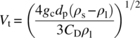
CD is the drag coefficient that can be estimated based on the hydrodynamic regimes, namely, laminar, intermediate, and turbulent, as shown in Table 11.3.
TABLE 11.3 Estimate of the Drag Coefficient CD Based on the Hydrodynamic Regime [6]
| Regime | Particle Reynolds Number ReP | Drag Coefficient CD |
| Laminar | ReP < 0.3 | |
| Intermediate | 0.3 < ReP < 1000 | |
| Turbulent | 1000 < ReP < 35 × 104 | CD = 0.445 |
11.3 MASS TRANSFER WITH CHEMICAL REACTION
In the previous section, we have discussed the mass transfer in the absence of reaction. In this section, we will introduce the complexity of chemical reaction. In Figure 11.1, we assumed dissolution of a solid‐phase A that is dispersed in a liquid solution. Now, let us assume bulk solution contain B at a certain concentration, CB, which reacts with A to form product P as shown in the Figure 11.3.
The overall reaction kinetics in the bulk phase are given by the following:
where
- kr is the reaction rate constant.
- CA and CB are the concentration of A and B in the bulk solution, respectively.
The reaction rate constant can be described by Arrhenius expression:
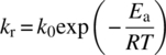
where k0, Ea, R, T are the Arrhenius pre‐exponential factor, activation energy, universal gas constant, and temperature in Kelvin, respectively.
An important point to note here is that none of the parameters in the equations describing reaction kinetics are related to reactor geometry. This is in contrast to what was observed earlier, for mass transfer dynamics, and the key reason why the Damköhler number can be used as metric relating the likelihood of scale sensitivity. We can see this, with greater clarity, coupling the reaction kinetic and mass transfer equations.
If we couple reaction kinetic in Eq. (11.11) with mass transfer in Eq. (11.2), we come to the following equation for the overall dynamics:
If we assume that B concentration is very high, we can assume its concentration is almost constant through the reaction we can replace kR = krCB, and Eq. (11.13) is further simplified to
At steady state ![]() , which means the transport rate equals the reaction rate:
, which means the transport rate equals the reaction rate:
Then, rearrange Eq. (11.15) and solve for CA:
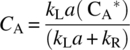
Then, substituted Eq. (11.17) from steady‐state approximation in Eq. (11.11), the following classical equation is obtained:

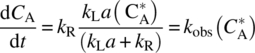
where kobs is the overall observable rate
Next, we will use Eq. (11.18) to understand the governing dynamics when mass transfer is coupled with a chemical reaction.
11.3.1 Very Fast Chemical Reaction: Regime 1
In the case where chemical reaction is very fast compared with mass transfer, i.e. kR ≫ kL, the denominator in the upper equation (kR + kLa) ≅ kR,
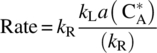
The upper equation shows that for mass transfer‐limited step coupled with a very fast chemical reaction, the overall observed rate is constant. A plot of concentration versus time will produce a straight line with a slope of ![]() . The latter correlation will be utilized in the case study (Section 11.4). In regime 1, the Damköhler number is high (Da > 100), and as discussed earlier, the observed rate is expected to be scale sensitive and dominated by mass transfer dynamics. Actually, Eq. (11.22) is strikingly similar to Eq. (11.2) with the exception that the solute concentration in the bulk liquid is assumed to be negligible, CA ≅ 0, which is expected under the current assumption of fast reaction. In other words, solute A never accumulates in the bulk and reacts as soon as it diffuses through the boundary layer. The overall system dynamics are dictated by the mass transfer dynamics, which are, in turn, influenced by the parameters that change with scale. Specifically, this is the scenario where the overall observed dynamics will be most sensitive to agitation, reaction geometry, and particle size. Therefore, special attention should be given to the particle size and to assurance that the stir speed is at or above the just‐suspended speed, see Section 11.2.2.2.
. The latter correlation will be utilized in the case study (Section 11.4). In regime 1, the Damköhler number is high (Da > 100), and as discussed earlier, the observed rate is expected to be scale sensitive and dominated by mass transfer dynamics. Actually, Eq. (11.22) is strikingly similar to Eq. (11.2) with the exception that the solute concentration in the bulk liquid is assumed to be negligible, CA ≅ 0, which is expected under the current assumption of fast reaction. In other words, solute A never accumulates in the bulk and reacts as soon as it diffuses through the boundary layer. The overall system dynamics are dictated by the mass transfer dynamics, which are, in turn, influenced by the parameters that change with scale. Specifically, this is the scenario where the overall observed dynamics will be most sensitive to agitation, reaction geometry, and particle size. Therefore, special attention should be given to the particle size and to assurance that the stir speed is at or above the just‐suspended speed, see Section 11.2.2.2.
11.3.2 Slow Chemical Reaction: Regime 2
In case where reaction rate is much slower than mass transfer kR ≪ kLa, Eq. (11.18) can be reduced to
The overall observed rate is predicted to be linear. A plot of overall observed rate will generate a straight line with a slope of ![]() . In regime 2, chemical reaction controls the overall observed system dynamics. The term kLa does not even appear on observed rate. In regime 2 Damköhler number is low. In this regime, increase in the agitation rate will not produce increase in the overall observed reaction rate. Indeed, for extremely slow reaction even complete suspension of the particles might not be necessary. Only gentle turnover for solids to prevent stagnant pockets inside the reaction is all what is needed. Reaction in this regime is not very sensitive to scale and tends to follow first principle reaction kinetics. In this regime with reaction kinetic control, the reaction is expected to be dependent on temperature based on Arrhenius equation (11.12) but not sensitive to scale assuming concentration and reagent equivalence were kept constant.
. In regime 2, chemical reaction controls the overall observed system dynamics. The term kLa does not even appear on observed rate. In regime 2 Damköhler number is low. In this regime, increase in the agitation rate will not produce increase in the overall observed reaction rate. Indeed, for extremely slow reaction even complete suspension of the particles might not be necessary. Only gentle turnover for solids to prevent stagnant pockets inside the reaction is all what is needed. Reaction in this regime is not very sensitive to scale and tends to follow first principle reaction kinetics. In this regime with reaction kinetic control, the reaction is expected to be dependent on temperature based on Arrhenius equation (11.12) but not sensitive to scale assuming concentration and reagent equivalence were kept constant.
11.3.3 Mass Transfer and Moderate Chemical Reaction: Regime 3
In the case where mass transfer and chemical reaction are occurring at a comparable rate, Eq. (11.18) cannot be further simplified as both terms contribute to the overall dynamics. In other words, one cannot decouple the rate of reaction from rate of diffusion.
11.3.3.1 Effect of Particle Size and Agitation Speed on the Overall Observed Rate in Regime 3
The effect of certain parameters such as agitation, particle size, and temperature is harder to predict in regime 3 when compared with regimes 1 and 2. However, we can look at the equation to understand the impact of several of the latter variables in these scenarios. Equation (11.18) shows that increase in the interfacial area, by reducing particle size, will increase the overall rate of reaction especially when mass transfer is contributing to the overall observed reaction. However, the increase will not be indefinite. In other words, at some point the particle size will be so small that mass transfer is much faster and reaction dynamics dominate, which is not a function of particle size, and thus the overall observed rate will plateau as the system moves from regime 1 to regime 2. Indeed, the latter conclusion is in agreement with experimental data, as shown in Figure 11.4a [8], where reducing particle size increased the overall rate. However, further reduction beyond approximately 2 mm did not improve the overall observed rate. In regime 2, particle size has a very little influence on the rate of reaction in the bulk.
FIGURE 11.4 Effect of (a) particle size and (b) agitation speed size on the overall observed rate.
Source: Adapted from Ref. [8].
In this regime, the impact of impeller speed is similar to that of particle size discussed above where increasing stirring speed is expected to increase the overall rate by increasing the fluid velocity and subsequently reducing the boundary layer film thickness; see Figure 11.3. Again, as with agitation, the increase will not be infinite according to Eq. (11.20) and at some point the reactions will not be mass transfer limited and dominated by reaction dynamics that is not a strong function of agitation rate; therefore, any further increase is predicted not to impact the overall observed rate. Indeed, as shown in Figure 11.4b, experimental data support the latter hypothesis. In the latter experiment, stirring speed increased the overall rate; however, at stirring speeds greater than 3600 rpm, the overall rates measured were essentially free of mass transfer limitations and independent of stirring speed.
11.3.3.2 Effect of Temperature on the Overall Observed Rate: Moving from Regime 2 to Regime 1
The temperature dependency of kR has been discussed using Arrhenius; see Eq. (11.12). Mass transfer coefficient kL can be explained by the fact that it is directly related to the solute diffusivity, D, Eq. (11.3). D can also be described by the Arrhenius equation as shown below:
where D0, ED, R, T are the Arrhenius pre‐exponential factor, activation energy of diffusion, universal gas constant, and temperature in Kelvin, respectively.
If one plots the logarithmic of the observable rate versus temperature, one would obtain a straight line whose slope is the reaction activation energy of the reaction, Ea, in regime 2, i.e. free of mass transfer limitation. On the other hand, in regime 1 where mass transfer dominates, the slope will be activation energy of diffusion, ED. However, the effect of temperature is typically modest, compared with reaction dependence. This week influence of temperature translates to a low/lower activation energy, ED. Activation energies for mass transfer limited are 10–20 kJ/mol compared with 40–60 kJ/mol for reaction processes. Therefore, an overall reaction can be slow, regime 2; however, with increasing temperature, the rate of reaction will accelerate, and eventually that reaction rate will be very fast and will be regime 1, i.e. mass transfer limited in which diffusion control, as shown in Figure 11.5.

FIGURE 11.5 Effect of temperature on the overall observed rate.
Source: Adapted from Ref. [2].
11.4 CASE STUDY: SCALING OF A MASS TRANSFER‐LIMITED REACTION
An early phase, API intermediate was planned to be run at a 250 L scale. The desired diaryl ether was formed via a SNAr reaction between the phenol (B) and fluorobenzonitrile (D) starting materials that were used in stoichiometric proportions with an excess of potassium carbonate base (A). The reaction was run in DMSO, where the starting materials were fully soluble and the potassium carbonate had sparing solubility. This heterogeneous reaction, depicted in Figure 11.6, had been developed on the bench scale to achieve yields of greater than or equal to 99% with a high purity profile with a reaction time of less than 12 hours.
FIGURE 11.6 Heterogeneous coupling reaction to form the diaryl ether, API intermediate.
Upon transfer of the process to the kilo scale facilities, the reaction was observed to take on the order of 4–5 times longer to achieve completion, prompting a root cause investigation. As discussed earlier, scale sensitivities are typically not associated with the chemical transformation, but the transport processes. In this case the chemical transformations were maintained but at a slower rate; there were no observations of an increase in the extent of competitive side reactions and no observable decomposition of the starting materials. In addition, the reaction could be accelerated to completion by additional charges of potassium carbonate. Further inquiry revealed that the grade of potassium carbonate was different than that used during development. The grade for the kilo‐scale run was purchased because it was more readily available and was a higher purity. However, upon inspection the particle size was noted to be larger, as seen in Figure 11.7. As discussed in Section 11.2, mass transfer dynamics is a very strong function of the interfacial area and thus the observed scale sensitivity pointed to mass transfer being the rate‐limiting step.
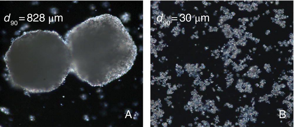
FIGURE 11.7 Polarized microscope images of potassium carbonate. Reaction completion was observed at 77 hours for material A and 12 hours for material B.
A short series of experiments were conducted to confirm the suspected cause and to develop a better understanding of the mass transfer limitation that could be used to set a strategy for future production activities. The general premise of these experiments was to exploit the relationship between reaction rate and particle size, or more specifically the surface area of potassium carbonate, to show the observed rate was controlled by the rate of mass transfer.
The experimental design involved preparing three portions of potassium carbonate with the same chemical purity but each with unique, well‐characterized size distributions such that the total area per unit mass was differentiable. This was accomplished by a combination of dry milling and sieving from one lot of potassium carbonate. This resulted in three distinct particle size distributions with areas per unit mass of 4902, 2387, and 1201 cm2/g as determined by Brunauer–Emmett–Teller (BET) analysis.
In instances where BET is not available, the surface area may sometimes be approximated from the particle size distribution through calculation within the particle size analyzer software using the appropriate moments of the distribution. Provided the particles are not of an irregular shape or highly aggregated, the estimates from the particle size distribution can be used in the mass transfer calculations. As seen within the table of Figure 11.8, this system has good agreement for the materials with the large and medium specific surface areas. However, the larger particles exhibited both agglomeration and irregular characteristics, leading to a deviation from the actual specific surface area and the estimate from the particle size distribution.
FIGURE 11.8 Particle size distribution for the smallest potassium carbonate and comparison of surface areas of the three portions using the PSD calculations and from BET measurement.
The coupling reactions were performed in parallel, where all conditions were kept equivalent with the exception of the particle size of potassium carbonate. Using three different particle size distributions of potassium carbonate, the reaction progress was monitored. The results of this are shown in Figure 11.9, where the conversion to product is plotted over time. In this example, off‐line samples were used to quantify the concentration of starting materials and the product by HPLC, but suitable PAT could have been used to increase the data density for regression of the kinetics and/or mass transfer characteristics. Attention was given to the agitation in these experiments to ensure the particles were fully suspended, stirring rate above Njs, such that the available surface area would not be a function of agitation performance as discussed in Section 11.2.2.2. This presented challenges for the largest size of potassium carbonate due to its large size and density. At reactor scales of less than or equal to 100 ml, the space between the reactor inner wall and the agitator was similar in size to the largest particle; thus uniform suspension was not possible without vigorous mixing that resulted in particle breakage. As a result, agitation was reduced such that partial suspension was achieved and onset of particle breakage was delayed. An inflection in the reaction profile was observed after approximately two hours as a result of particle breakage, which was conferment via microscopy.
FIGURE 11.9 Reaction conversion profiles for the diaryl ether formation using potassium carbonate with three different particle size distributions. Conversion on the y‐axis is equal to the moles of product at the sampling point divided by the moles of limiting substrate multiplied by 100.
This case study resembles the scenario described in Figure 11.1 where K2CO3 is (A) suspended in an agitated vessel. Starting from general Eq. (11.13) to describe the role of K2CO3,
Based on the magnitude that conversion was impacted by the particle size of the potassium carbonate, it was decided to start the regression from assumption that the mass transfer rate was the rate‐limiting step for the reaction. More specifically the rate of reactions (R2 and R3) was significantly faster than the rate of mass transfer (R1). Initially, while substrates are in high concentration, the reaction is assumed to be fast, leading to the approximation that in the initial period CA ≈ 0 because it is being converted to product (P) as fast as it is available in solution:
and
As the potassium carbonate was in excess at 304 mg/ml with sparing solubility of approximately 47 mg/ml [9], an additional assumption was made that the surface area was constant, allowing the data to be regressed in the initial period as shown in Figure 11.10.
FIGURE 11.10 Observed rates of reaction for the initial period where the rate is controlled by mass transfer for the three different sizes of potassium carbonate.
Comparison of the relative rates for the initial period leads to three observations:
- Mass transfer is proportional to surface area for the conditions where the particles were well suspended. From Figure 11.8 it is observed that the ratio of surface areas for the small and medium particles is 2.05. Under the applied assumptions we would expect the relationship of the mass transfer rates to be the same ratio. From Figure 11.10 we see the rate for the small particles is 2.84 × 10⁻⁷ mol/(ml s) and that of the medium particles is 1.39 × 10⁻⁷ mol/(ml s), giving a ratio of 2.04.
- The slope for the largest particle was expected to be half of that of the medium particles, i.e. 0.7 × 10⁻⁷ mol/(ml s). However, the observed rate was almost eight times lower than expected from the impact of area alone. The issues with the largest particle size are related to operating below full suspension. This is consistent with the mass transfer rate relationship with mixing as highlighted in Figure 11.2, where the mass transfer rate is decreased significantly when operating below complete suspension. Thus, highlighting the significance of ensuring agitation is well above the Njs during production.
- Surface area has not been increased to the point where mass transfer was no longer a rate‐limiting step. As depicted in Figure 11.4a, surface area can be increased to a point at which mass transfer may no longer be the limiting rate for the overall observed rate and therefore no change in rate as the area increased. In this case, the area did not reach that point. However, there is a practical limitation to decreasing the particle size for this application. Namely, the value of further reduction is limited as the reaction is complete in less than six hours for the smallest particles and to reduce the particle size significantly lower than that used in this study would require specialty milling equipment, increasing cost and complexity to the process.
To ensure that these results were not appreciably impacted by mixing above the power necessary to fully suspend the solids, additional data was gathered at high and low mixing speeds and at a scale change greater than one order of magnitude. In all instances the results are consistent with the observed rates on Figure 11.10.
This knowledge was used to introduce a milling step for potassium carbonate in the kilo‐scale run and define a raw material specification for the pilot plant that balance the reaction time with commercially available materials. In the case of the kilo scale runs, the resulting particle size from milling was used to predict a reaction time of 6.5 hours, in agreement with the observed reaction times of 6.5–7 hours. The particle size specified for the pilot scale predicted a reaction time of 12 hours, identical to the time observed on scale.
11.5 NOTATIONS
| a | Interfacial area | |
| CA | Concentration of solute A | |
| CB | Concentration of solute B | |
| Saturation concentration of A, solubility limit | ||
| CD | Drag coefficient | n/a |
| D | Solute diffusivity | |
| D0 | Diffusivity Arrhenius pre‐exponential factor | |
| Da | Damköhler number | n/a |
| Dimp | Impeller diameter | m |
| dp | Particle diameter | m |
| Ea | Activation energy | |
| ED | Activation energy of diffusion | |
| gc | The gravitation constant | |
| k0 | Arrhenius pre‐exponential factor – first order | |
| kL | Mass transfer coefficient | |
| kobs | The overall observable rate | |
| kr | The reaction rate constant | |
| kR | Observed reaction rate kr[CB], assuming CB is in excess and not changing during the course of reaction | |
| δ | Boundary layer | m |
| Njs | Just‐suspended speed | rps |
| μl | Viscosity of the bulk liquid, respectively | Pa ∙ s |
| ρl | Bulk liquid density | |
| ρs | Solid density | |
| ReP | Particle Reynolds number | n/a |
| S | Dimensionless number that is a function of impeller type | n/a |
| Sc | Schmidt number | n/a |
| T | Temperature | Kelvin |
| Vm | Molar volume of diffusing species at its boiling point | m3/mol |
| Vt | Free settling velocity | |
| X | The mass ratio of suspended solids to liquid time 100 | n/a |
10.5 ACKNOWLEDGMENTS
The authors of this chapter would like to acknowledge and thank the following for their contributions to the preceding text: Daniel Griffin, Kenneth McRae, Jacqueline Milne, Scott Roberts, Shawn Walker, and Margaret Faul.
REFERENCES
- 1. Hulshof, L.A. (2013). Right First Time in Fine‐Chemical Process Scale‐Up: Avoiding Scale‐Up Problems: The Key to Rapid Success. Mayfield, U.K.: Scientific Update LLP.
- 2. Fogler, H.S. (2000). Elements of Chemical Reaction Engineering, Prentice Hall International Series, 4the. Upper Saddle River, NJ; London: Prentice Hall PTR.
- 3. Harnby, N., Edwards, M.F., and Nienow, A.W. (1992). Mixing in the Process Industries, 2nde. Oxford: Butterworth‐Heinemann.
- 4. Houson, I. (2011). Process Understanding: For Scale‐Up and Manufacture of Active Ingredients, 1ste. Weinheim, Germany: Wiley‐VCH.
- 5. Mohan, A.E., Kukura, J., Spencer, G., and Ulis, J. (2015). Solid–Liquid Suspension in Pilot Plants: Using Engineering Tools to Understand At‐Scale Capabilities. Organic Process Research & Development 19 (9): 1128–1137.
- 6. Paul, E.L., Atiemo‐Obeng, V., and Kresta, S.M. (2003). Handbook of Industrial Mixing: Science and Practice. New York: Wiley.
- 7. Perry, R.H. and Green, D. (1984). Chemical Engineer's Handbook. New York: McGrow‐Hill.
- 8. Davis, M.E. and Davis, R.J. (2003). Fundamentals of Chemical Reaction Engineering. New York, NY: McGraw‐Hill Higher Education.
- 9. Cella, J.A. and Bacon, S.W. (1984). Preparation of Dialkyl Carbonates via the Phase‐Transfer‐Catalyzed Alkylation of Alkali Metal Carbonate and Bicarbonate Salts. The Journal of Organic Chemistry 49 (6): 1122–1125. https://doi.org/10.1021/jo00180a033.