
12
SCALE‐UP OF MIXING PROCESSES: A PRIMER
Francis X. McConville and Stephen B. Kessler
Impact Technology Development, Lincoln, MA, USA
12.1 INTRODUCTION
The problems associated with the scale‐up of mixing processes are universal. This is because the dynamics and mechanics of liquid agitation and blending are often poorly understood, and yet these operations play a fundamental role in many aspects of the chemical and pharmaceutical industries. The success of homogeneous and heterogeneous chemical reactions, crystallizations, liquid–liquid extractions, and so many other operations is critically dependent on effective mixing and appropriately designed mixing systems. Unfortunately, as we shall see below, duplicating the energy and quality of mixing available in the laboratory at commercial scale can prove extremely difficult.
For example, the motor power required to turn agitators increases exponentially as the diameter of the agitators increases, making it prohibitively expensive to match, one to one, the mixing power input of small‐scale reactors in large commercial vessels. This results in batch blend times, the time it takes for the contents of a batch reactor to become homogenized, sometimes orders of magnitude longer in commercial reactors than in the laboratory. This can have severe consequences for the results of many chemical operations.
Frequently, heterogeneous reactions such as catalytic hydrogenations fail to achieve expected reaction rates upon scale‐up because there is insufficient mixing to fully suspend the catalyst particles. The catalyst settles to the bottom of the vessel where it is inaccessible to the reactants in solution and therefore cannot effectively catalyze the reaction.
Differences in local and average shear conditions due to differences in impeller diameter and impeller tip speeds in commercial vessels can have unexpected consequences for shear‐sensitive processes such as fermentations using living cells or crystallization of materials that require a specific particle size distribution. High shear can also cause severe emulsification at large scale that might not have been experienced in the lab.
These are just a few of the types of problems often encountered at large scale due to the fact that mixing conditions differ so much from those available in the laboratory. Mixing scale‐up often proves to be a compromise between cost and performance and between achieving the desired result and minimizing unexpected negative effects. The better the understanding of the fundamental principles of mixing and of the specific requirements of the process involved, the better the results of this compromise will be.
12.2 BASIC APPROACHES TO MIXING SCALE‐UP
Over the years, scientists and engineers have considered many approaches to scaling up mixing processes, with the ultimate goal of successfully matching laboratory results at commercial scale at a reasonable cost. As a result, numerous scale‐up parameters, equations, and principles have been developed, some of which work better or are more reliable than others depending on the specific application. No single method has been successful for all situations, and the characteristics of the system must be understood as well as possible to maximize the chances for success.
12.2.1 Principles of Similarity
Modeling theory considers two processes similar if they possess geometric, kinematic, and dynamic similarity. Geometric similarity requires that linear dimensions of two systems are scaled by the same ratios at different scales. Kinematic similarity requires geometric similarity and also that characteristic velocities scale by the same ratio. Dynamic similarity requires both geometric and kinematic similarity and adds the requirement that characteristic forces scale by the same ratio.
Rigorous application of modeling theory is rarely applied to scale‐up of industrial mixing processes. One reason for this is that when more than two force properties are important in a mixing process, full dynamic similarity cannot be achieved. Since most mixing processes involve three or more force properties, a choice must be made among the possible properties to select one as a scaling factor. This choice is made by considering the nature of the process at hand and applying scaling factors that have been proven to work in similar processes. Some commonly used approaches to mixing scale‐up and their utility in specific situations are described in the following sections.
12.2.2 Geometric Similarity
The concept of geometric similarity is illustrated in Figure 12.1. Adhering to geometric similarity can be extremely important in designing systems for scale‐up or for building small‐scale experimental vessels designed to mimic the behavior of a larger system for research purposes. This latter approach, called scaling down or modeling, is an important aspect of mixing engineering and widely used to study the mixing behavior of commercial systems at a more convenient scale.
FIGURE 12.1 The principle of geometric similarity for stirred tanks. Key ratios (D/T, C/T, B/T, Z/T) are held equal at both scales. (B, baffle width; C, impeller bottom clearance; D, impeller diameter; T, tank diameter; Z, liquid height.)
Figure 12.1 shows how certain key ratios would be held equal in two geometrically similar vessels of different sizes. Thus the ratio of impeller diameter to tank diameter (D/T) is identical in both cases, as are the ratios of the liquid level (Z), the impeller bottom clearance (C), and the baffle width (B) to the tank diameter.
A number of practical issues limit the usefulness of this technique alone as a primary scale‐up method. Firstly, mechanical limitations may limit its utility in some cases. For example, marine impellers are often used in laboratory systems. However, in large‐scale industrial mixing applications, these impellers are impractically heavy if scaled up by geometric similarity. Also, the shape of the vessel heads is usually not limited by mechanical considerations in the laboratory, but in most industrial applications, vessel head design is defined by codes that take mechanical stresses into account. These types of limitations can sometimes be overcome by anticipating large‐scale design issues and creating scaled‐down laboratory vessels that match the large‐scale geometry.
In addition to such limitations in the application of geometric similarity, there are limitations in what can be achieved when it is applied. Due to the rules of geometry, as a vessel doubles in diameter, its volume increases by a factor of 8 (23). Thus, when scaling up by a factor of 2, it is not possible to maintain certain key ratios such as surface area per unit volume or the volume/diameter ratio. It also proves impossible to operate these two systems in such a way that the intensity of mixing (as measured by power input per unit volume, P/V, for example) and the velocity of fluid circulation are both identical. It is possible to design and operate two systems of different sizes at an identical P/V, but the fluid circulation patterns, fluid velocities, degree of turbulence, etc. would likely be very different. If a successful process result relies on a particular fluid motion, it might not be achieved upon scale‐up by simply maintaining geometric similarity and matching P/V. Such limitations are the source of much confusion and difficulty. In most cases, geometric similarity proves to be useful as a starting point for scale‐up, but several other factors must be considered to ensure success.
Consequently there are situations where deliberate deviation from geometric similarity is the best approach to scale down. Oldshue [1] uses the term “nongeometric similarity” to describe a situation where conventional concepts of similarity must be sacrificed so that certain factors can be controlled to achieve successful scale‐up. For example, with geometric similarity observed, a scaled‐down vessel could be operated at the same tip speed as its full‐scale counterpart, but this requires that the impeller in the scaled‐down vessel be operated at higher rpm. In this example, the maximum shear rate in the two vessels is the same, but the average shear rate in the impeller region is higher in the small vessel. If shear rate is one of the key process variables being modeled, the mismatch in maximum and average shear rates can be reduced by increasing the diameter of the impeller in the scaled‐down vessel relative to the vessel diameter (D/T). Tip speeds will now match at lower rpm in the small vessel, which would correlate with a smaller difference in impeller average shear rate.
More detailed information on system geometry and the application of geometric similarity to mixing processes can be found in Uhl and Von Essen [2] and Johnstone and Thring [3].
Figure 12.2 shows some typical “shape factors” – geometric ratios that have historically proven effective in systems designed for mixing processes and can be used as a general guide to vessel design. For example, many mixing vessels employ agitators with diameters approximately 1/3 of the vessel diameter, located one impeller diameter off the bottom. Again, these values are typical but can vary significantly in equipment designed for specific applications.

FIGURE 12.2 Typical shape factors, or geometric ratios, found useful for general mixing applications in stirred tanks.
12.2.3 Rate of Turbulent Energy Dissipation and P/V
A particularly useful and widely used approach to mixing scale‐up involves maintaining a constant rate of turbulent energy dissipation, ε, across the various scales. ε, which is defined by Eq. (12.1), is usually expressed in units of W/kg:
where
- P is power input (W).
- ρ is liquid density (kg/m3).
- V is liquid volume (m3).
ε is fundamental in describing the interrelationship between turbulence and mass transfer in mixing operations. This statement is illustrated by the Kolmogorov length scale, which characterizes the smallest eddies associated with turbulent mixing. The Kolmogorov eddy length η is defined by Eq. (12.2), where ν is kinematic viscosity:

At the length scale represented by η, viscous forces in the eddy are equal to inertial forces due to turbulent velocity fluctuations. The Kolmogorov eddy length underlies and informs the use of ε as a scaling parameter. Kinematic viscosity, ν, is a liquid property that is scale independent; thus constant ε is sufficient to fix a value for η over a range of scales. However, it remains to define the region for which ε is applicable. A mean value of ε can be calculated from the total power input and mass of liquid in the vessel. This overall mean value of ε is useful where an operation is governed by bulk flow characteristics. For geometrically similar vessels, it is sometimes assumed that holding overall mean ε constant is sufficient to provide accurate scaling in the impeller region. For more accurate scaling of local characteristics, a better approach is to define a volume based on the swept volume of the impeller instead of the total batch volume. A method for calculating impeller swept volume is given in Kresta and Brodkey [4].
Another parameter that is used to represent average mixing intensity in a vessel is power/unit volume (P/V). P/V is sometimes called power intensity and is usually expressed in either W/l or HP/1000 gal. In scaling equations that involve ratios of ε or P/V to represent different sizes of equipment, either ε or P/V works equally well. However, because of its units, P/V cannot be applied in fundamental equations that define turbulence and mass transfer in mixing systems. Also keep in mind that in large vessels, local values of ε may vary widely in different regions of the vessel.
When mean values of either ε or P/V are used for scale‐up, it is important to also maintain geometric similarity. This is because in some mixing applications, a local value of ε may be of greater importance than the vessel average value. This point is well made in Figure 12.3, which shows three vessels all operated at the same P/V, but the fact that their geometries are very different (specifically impeller size) results in very different results in the suspension of solids. The effects shown are the result of calculations made with the commercial computational fluid dynamics (CFD) program VisiMix® [5].

FIGURE 12.3 These three cases illustrate the importance of system geometry and the distinction between mean rate of energy dissipation (ε) and maximum local rate of energy dissipation. While all three vessels are operating at the same average value of ε, differences in geometry result in very different fluid motion and mixing behavior, in this case manifested by differences in the suspension of solids as predicted by VisiMix [5].
As shown in Eqs. (12.3) and (12.4), ε and P/V can be expressed in terms of the impeller diameter D, its rotational speed N, liquid volume V, batch density ρ, and a parameter called the power number NP that is explained in more detail below:
Power number, Np, is a dimensionless number characteristic of a given impeller and vessel geometry. It is defined by Eq. (12.5):
Figure 12.4 lists some typical values of power number for various types of impellers, but geometric factors such as impeller tip chord angle, number of blades, position of the impeller within the vessel, and the number and dimensions of baffles all affect the value of the power number. For this reason, accurate power number values for a particular system can only be obtained experimentally, by measuring power draw via a wattmeter, or, more accurately, by directly measuring torque on the impeller shaft, under well‐defined experimental conditions.
FIGURE 12.4 Typical power numbers (NP) for various impeller types. These values are only approximate as the power number is significantly affected by number and pitch of blades, tip chord angle, position of the impeller within the vessel, baffle configuration, and other geometric factors.
As in any type of fluid flow, fluid motion in mixing can be generally classified as either turbulent or laminar, depending on the velocity and other physical parameters. A common term for quantifying this is the impeller Reynolds number NRe, a dimensionless parameter defined by Eq. (12.6). Values of NRe can range from single digits for highly viscous flow to hundreds of thousands for very turbulent flow:
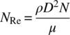
At impeller Reynolds numbers greater than about 104, fluid motion is considered turbulent, and under such conditions, the power number NP assumes a constant value. Under laminar mixing conditions (NRe < 100) and in the transitional regime between laminar and turbulent mixing, power number varies, typically increasing with decreasing Reynolds number as shown by the curves in Figure 12.5. The values of NRe that delineate the transitional region are only approximate and will vary depending on the system.
FIGURE 12.5 Relationship between impeller power number NP and impeller Reynolds number NRe for some typical impeller types. At NRe > 104, flow is turbulent and NP reaches a constant value. The power number generally increases under laminar conditions (NRe < 10) and in the transitional regime between laminar and turbulent.
Source: Adapted from Hemrajani and Tatterson [6] and Rushton [7].
Note that the fluid viscosity term does not appear in the equations that define ε or P/V, but is captured indirectly in this relationship between power number and Reynolds number. It should be assumed that published values such as those given in Figure 12.4 represent turbulent power numbers. It is usually necessary to use empirical relationships such as those shown in Figure 12.5 to estimate NP values under nonturbulent conditions.
The importance of the power number NP and its application in typical mixing calculations are illustrated in Example Problem 12.1.
Example Problem 12.2 illustrates the basic approach for scaling up by maintaining constant mean rate of energy dissipation, ε, in two vessels of different scales.
12.2.4 Tip Speed
Tip speed is simply tangential velocity of the impeller at its maximum diameter and is calculated according to Eq. (12.7):
Tip speed is related to maximum shear rate in stirred vessels. For this reason, tip speed is often applied as a scaling parameter for operations where maximum shear is a critical determinant of the process outcome. This includes those processes for which shear can be either beneficial or detrimental. This issue is discussed in more detail in the section on shear below. When vessels are scaled according to geometric similarity and at constant mean energy dissipation rate, tip speed will be higher in the larger vessel, a fact supported by Eq. (12.7).
In addition to its relationship to maximum impeller shear, in geometrically similar vessels, tip speed scaling corresponds exactly to scaling at constant torque per unit volume. In fully turbulent flow, i.e. above NRe = 104, all velocities scale with tip speed regardless of viscosity. Because of these relationships, tip speed or torque per unit volume is useful in scaling mixing processes that are controlled by flow such as blending of miscible liquids and suspension of solids in liquids.
12.2.5 Blend Time
Blend time is an empirical factor that describes the time it takes for the contents of a vessel to become homogenized, particularly important during chemical additions to a batch. It is usually determined experimentally by monitoring the dispersion of a dye or other tracer compound, either visually or by means of detection probes located at various points in the vessel.
Often, an acceptable blend time is established based on a practical, realistically achievable value such as 99% uniformity. Although somewhat subjective, blend time is a critical factor in the scale‐up of many operations, particularly rapid chemical reactions that rely on rapid dispersion during controlled addition of a reagent. This is discussed in detail in the section on mixing‐limited reactions below.
Figure 12.6 illustrates that blend time increases rapidly when P/V is held constant but vessel size increases. Holding blend time constant with increasing vessel size requires maintaining constant impeller speed in geometrically similar vessels. This approach leads to increasing P/V with vessel size and, ultimately, to unrealistically high power requirements. Values much higher than 1–2 W/l are difficult to achieve in standard stirred tanks at large scale as beyond that, motors would become impractically large.
FIGURE 12.6 Relationship between blend time and vessel volume for various levels of power input (P/V).
Impeller design and number of impellers will also have a significant effect on blend time. Some types of impellers, such as standard anchor blade impellers, which are not designed for good bulk mixing, generally result in very long blend times, whereas a pitched blade turbine operated at typical speeds in the same vessel would result in much shorter blend times.
Various correlations have been developed to help maintain constant blend time at different scales, such as the translation equations introduced below, but their success depends heavily on impeller design and other geometric factors. For standard vessel and impeller geometries, correlations are available that estimate blend times for the turbulent, transitional, and laminar regimes [8].
In mixing calculations, it is common to see a variable called “dimensionless blend time,” which is essentially the product of the actual blend time and the impeller rotational speed, although often other geometric factors are included in equations used to calculate it.
12.2.6 Shear
As mentioned earlier, shear in a batch mixing operation can have desirable or undesirable effects, depending on the intended result of the operation. For example, maintaining sufficiently high shear rate in the impeller region may be required to rapidly disperse a reactant being fed into a vessel during a chemical reaction. However, the product of this same reaction may be a solid precipitate whose particles are shear sensitive and would suffer attrition, creating fines and complicating downstream recovery if high shear rates are maintained for too long.
Controlling shear rates when such a process is scaled up can become a complex undertaking. Various correlations presented in the literature to estimate shear rates in mixing vessels predict a broad range of shear rate values. Moreover, shear rates may be predicted to increase, decrease, or remain constant on scale‐up, depending on the shear correlation and scale‐up approach that are chosen. Some examples of the available correlations are described below.
One widely used correlation, the Metzner–Otto relationship, predicts average shear rate in the impeller region. This relationship, defined by Eq. (12.8), is valid for laminar, transitional, and moderately turbulent conditions:
where
-
 Z is shear rate in per second.
 - k′ is a dimensionless Metzner–Otto coefficient characteristic of the impeller.
- N is impeller speed in rev/s.
For a Lightnin® A310 hydrofoil impeller (see Figure 12.4), the value of k′ is 8.6. Thus the estimated average shear rate in the impeller region for an A310 running at 100 rpm is
The value of shear rate predicted by the Metzner–Otto relationship depends only on impeller type and speed and is independent of impeller and vessel dimensions.
To estimate maximum shear rates produced in the flow near the impeller tip, an approach analogous to the Metzner–Otto relationship is used. In this case, a single value of the coefficient, k′ = 150, is applied regardless of the impeller type. For estimating maximum shear on the impeller surface, a value of k′ = 2000 is sometimes applied.
As mentioned in the section on tip speed, this factor can be related to maximum shear rate near the impeller tip. While the k′ = 150 rule described above applies for moderate Reynolds number (laminar and transitional) conditions, tip speed is recommended for higher NRe conditions as a means of scaling on the basis maximum shear rate. There is no general rule found in the literature that correlates tip speed with shear rate. When used for scaling purposes, tip speed is held constant as scale increases, which is assumed to provide constant maximum shear rate.
For estimates of shear rate averaged throughout a vessel under turbulent conditions, a vessel average shear rate can be calculated based on total energy dissipation. Eq. (12.9) defines this correlation:
As described above, the various shear rate correlations provide widely divergent values on scale‐up. To illustrate this point, Figure 12.7 compares the shear correlations that are presented above. The graph presented in Figure 12.7 covers a range of 100 : 1 scale‐up of impeller diameter under the condition of geometric similarity, which corresponds to a range of 106 : 1 in vessel volume. ε and P/V are held constant. Under these conditions, shear rates in the impeller region, in the flow near the tip, and on the tip surface, which are each defined by a constant multiplied by rpm, all decrease with increasing impeller diameter. Vessel average turbulent shear rate remains constant when P/V is held constant. Tip speed as an indicator of shear rate increases with increasing impeller diameter at constant P/V.

FIGURE 12.7 Theoretical effect of scale on various manifestations of shear in a mixing vessel under conditions of geometric similarity and constant ε (and P/V). Shear rates in the region swept by the impeller, in the flow near the tip, and on the tip surface, which are each defined by a constant multiplied by rpm, all decrease with increasing impeller diameter. Vessel average turbulent shear rate remains constant under these conditions. Tip speed as an indicator of shear rate increases with increasing impeller diameter.
General guidelines in the literature indicate that Metzner–Otto‐type correlations are best applied over the laminar and transitional Reynolds number ranges. Vessel average shear applies only under fully turbulent conditions. Tip speed can be used as a scaling factor for maximum shear under fully turbulent conditions. However, these guidelines should not be relied upon if a process is to be scaled up in which shear is an important consideration. In this case, lab‐ and pilot‐scale experiments should be conducted to evaluate the effects of shear over a range of scales whereby a correlation can be selected for commercial scale‐up.
12.2.7 Scaling (Translation) Equations
In keeping with the concept of similarity, a number of relationships, sometimes called translation equations, are used in an attempt to match operating conditions at two different scales. Various authors have developed different approaches for different situations.
For example, the equations below illustrate some relationships that have been proposed for maintaining equal blend time between small‐scale and large‐scale vessels for batch mixing operations [9]:


The application of translation equations such as these depends very much on the specific application and system geometry, and as always experimental validation at two different scales is strongly recommended when applying them to predict performance in commercial‐scale operations. A wide array of translation equations used for various purposes under various conditions is examined by Uhl and Von Essen [2].
12.3 OTHER CONSIDERATIONS IN MIXING SCALE‐UP
12.3.1 Importance of Fluid Rheology
While Reynolds number is seldom used as a mixing scale‐up correlation per se, knowing whether a mixing operation is conducted under laminar, transitional, or turbulent flow conditions is vital to successful scale‐up. For example, if the commercial‐scale operation will be fully turbulent, then lab‐ and pilot‐scale experiments must be designed to operate under turbulent conditions as well. Liquid viscosity is a primary determinant of the value of impeller Reynolds number, defined by Eq. (12.6), so knowledge of the viscosity that is characteristic of a given mixing operation is vital as well.
If an operation comprises blending of Newtonian liquids or suspending an immiscible solid in a Newtonian liquid, then obtaining the required viscosity data is straightforward. The liquids may have well‐known viscosities that can be found in literature references. If not, then measurement of Newtonian viscosity is a simple matter that can be performed with inexpensive instruments. However, if the liquid being mixed contains macromolecular solutes or colloidal‐size particles, it may exhibit non‐Newtonian characteristics. In this case, defining its rheology requires more than a single coefficient, and measurements may require more sophisticated instruments and techniques.
The flow properties of a Newtonian liquid are defined by Eq. (12.12):
where
- τ is shear stress.
- μ is coefficient of viscosity.
-
 is shear rate.
Shear‐thinning fluids are often encountered when dealing with macromolecular solutes or colloidal suspensions. Such fluids can be effectively modeled by a power law, shown in Eq. (12.13):
where
- K is a consistency index.
- n is a behavior index.
If a shear‐thinning fluid also exhibits a yield stress (i.e. there exists a shear stress below which no flow occurs), then the Herschel–Bulkley model, shown in Eq. (12.14), can be applied:
where
- τ0 is yield stress.
Mixing of yield stress fluids can prove particularly challenging to scale‐up. If the yield stress is of sufficient magnitude, then use of a conventional turbine‐style impeller may result in a well‐mixed cavern of liquid surrounding the impeller with little or no liquid motion closer to the vessel walls. In this case, a close‐clearance impeller that sweeps close to the walls of the vessel, such as an anchor or helical ribbon, may be required. Empirical correlations are available to assist with these scale‐up problems. These correlations are specific to impeller geometrical factors, and their efficacy will depend on choosing an appropriate rheological model and thorough characterization of the fluid.
Rheological models exist for many known types of fluid behavior. In addition to the non‐Newtonian behaviors discussed above, additional levels of complexity such as time dependency and viscoelasticity can also be modeled. To support such models, measurement of the properties of non‐Newtonian fluids requires the use of a rheometer. Rheometers are capable of controlling either shear stress or shear rate applied to a sample and are adaptable to multiple test geometries. A detailed discussion of non‐Newtonian rheometry is beyond the scope of this chapter. A recommended reference in this regard is Macosko [10]. A particularly powerful combination of techniques for scaling of mixing operations for non‐Newtonian fluids is the use of appropriate rheological models in conjunction with CFD as described in a later section.
12.3.2 The Role of Mixing in Heat Transfer
Heating and cooling batch vessels is a fundamental operation in any chemical processing endeavor. The rate and efficiency of heat transfer in and out of such vessels depend on many things, including the intrinsic heat transfer coefficient of the system, the temperature difference between the batch contents and the heat transfer medium (such as the fluid in the vessel heating jacket), and certain key properties of the batch itself (such as density, thermal conductivity, and heat capacity).
However, mixing also plays a major role in determining heat transfer efficiency. While a full treatment of heat transfer in agitated vessels is beyond the scope of this chapter, it is worth pointing out some fundamental principles.
A common dimensionless group that characterizes process‐side heat transfer in stirred tanks is the Nusselt number NuL, which is a measure of the ratio of convective heat transfer to conductive heat transfer. It is defined in Eq. (12.15):
where
- hi is the process‐side heat transfer coefficient,
- D is the vessel diameter, and
- k is the thermal conductivity of the batch.
The value of NuL is strongly dependent on the mixing Reynolds number. NuL values close to unity indicate sluggish motion and heat transfer driven primarily by thermal conduction. Under highly turbulent conditions, NuL values can range from 100 to 1000, which indicates highly efficient convective heat transfer. Thus providing a sufficient degree of mixing is an important factor in designing vessels that will be used for heating and cooling. Many very comprehensive texts on process heat transfer are available for additional information, such as Serth [11].
12.3.3 Continuous Mixing Scale‐Up
While a majority of mixing operations in the pharmaceutical industry are still performed in batch mixing vessels, there is a trend toward instituting continuous processing. This trend is being fostered by the FDA through elimination of regulatory constraints that previously limited most pharmaceutical process to the batch approach. The advantages of continuous mixing include potentially much higher productivity and improved heat transfer, mass transfer, and mixing. The latter three advantages are attributable primarily to reduced mixing volume.
Current examples of continuous mixing processes in the pharmaceutical industry mainly involve mixing‐sensitive chemical reactions, that is, fast consecutive reactions that occur on a time scale that is short compared with practical blend times for commercial‐scale batch mixing vessels. Most of the reactors used for these operations are of tubular configuration – for example, in‐line static mixers. The continuous stirred tank reactor (CSTR) is also used and may find new applications with the current regulatory environment favoring continuous processes.
The typical objective of batch mixing operations is to achieve a spatially homogeneous mixture within a fixed process volume, within a specified blend time. Continuous mixing operations are designed to produce a spatially and temporally homogeneous effluent stream within a specified residence time. While blend time is the key parameter characterizing batch mixing operations, residence time distribution (RTD) is the key parameter characterizing continuous operations. Figure 12.8 plots the response of a sensor at the outlet of a mixing vessel to a step input of tracer at the inlet. The two RTD curves illustrate ideal flow patterns that establish the bounds within which real stirred tanks operate: the plug flow reactor (PFR) and the CSTR. A PFR represents the unmixed limit or complete segregation, while the ideal CSTR represents perfect macromixing.

FIGURE 12.8 The response of a sensor at the outlet of a mixing vessel to a step input of tracer at the inlet for both plug flow reactors (PFR) and continuous stirred tank reactors (CSTR). The two ideal retention time distribution (RTD) curves illustrate the bounds within which real stirred tanks operate.
The y‐axis parameter in Figure 12.8, FCSTR = A/A0, is the concentration of tracer measured at the outlet (A) divided by the concentration applied at the inlet (A0). The parameter θ in Figure 12.8 is dimensionless residence time, defined by Eq. (12.16):
where
-
 is the mean residence time (vessel volume/flow rate).
 - t is time elapsed following application of tracer.
In the case of plug flow (dotted curve), no tracer is detected at the outlet until θ = 1, at which point the tracer concentration jumps to the value at the inlet. For the CSTR (solid curve), when tracer enters the vessel, some is detected instantly at the outlet, and its concentration continues to rise exponentially, approaching asymptotically the inlet concentration (see Eq. (12.17)):
Real stirred tanks are often assumed to behave as ideal CSTRs. However, some degree of nonideal flow is likely to occur due to channeling, recycling, stagnant regions, or a combination of these effects. In many cases a real stirred tank may approximate the ideal CSTR closely enough that deviations from ideal flow have a negligible effect on the process. However, such deviations must be considered when scaling up. To quote Levenspiel [12], “The problems of nonideal flow are intimately tied to those of scale‐up…Often the uncontrolled factor in scale‐up is the magnitude of the nonideality of flow, and unfortunately this very often differs widely between large and small units. Therefore ignoring this factor may lead to gross errors in design.”
For purposes of design and scale‐up of continuous mixing operations, the ratio of the mean residence time in a CSTR divided by the batch blend time for the same vessel is defined by Eq. (12.18):
where
- V is mixed volume.
- Q is flow rate through the vessel.
- Θ is the batch blend time for the vessel, which is either measured or estimated.
To ensure continuous mixing that is near‐ideal CSTR in character, a rule of thumb states that the ratio α should be greater than 10. The basis for this ratio is discussed by Roussinova and Kresta [13].
In addition, the location of inlet and outlet ports must be considered. The rule to be followed in this regard is that a straight line drawn from the inlet port to the outlet port should pass through the impeller(s).
Scaling of the ratio of inlet flow to the impeller flow must also be considered. The simplest approach is to limit the average velocity of the liquid in the inlet port to be less than the tip speed of the impeller. Recommended ranges for this ratio can be found in Hemrajani and Tatterson [6]. Ratios of momentum and specific energy dissipation between the entering liquid jet and the impeller flow are sometimes used as scaling factors instead of a velocity ratio. These scaling approaches are also frequently applied in semi‐batch mixing, which is discussed in Section 12.2.3.
Scale‐up of static mixers for use in continuous mixing processes is beyond the scope of this chapter. See Etchells and Meyer [14] for further reading regarding this topic.
12.4 COMMON MIXING EQUIPMENT
Because of the wide variety of mixing processes encountered in the industry, a great number of mixing types and geometries have been developed, including fluidized beds, jet nozzles, and gas sparging. Here however, we will focus on mechanically stirred tanks and examine the typical impeller types used in this application. Such stirred vessels are used for batch production of the vast majority of specialty chemicals and pharmaceuticals, for blending and homogenization, for creating dispersions, and for running chemical reactions.
12.4.1 Major Impeller Types Used in Batch Mixing
Batch vessels may employ a broad range of impeller designs, each optimized for a particular type of process duty. The impellers shown in Figure 12.4 are among the more common types used in agitated vessels in chemical processing. Some vessels use multiple impellers of different types on a single shaft to obtain better mixing results. For example, it is common to utilize a high‐shear flat‐blade turbine at the bottom and a high‐flow pitched blade impeller higher up the shaft in certain blending and dispersion operations.
Based on their design, impellers can be broadly categorized as generating an axial flow pattern or a radial flow pattern. In the case of a stirred tank, the axial flow pattern results in a pumping action, usually downward, that is very useful for preventing the settling of solids and generating good cross‐mixing. Examples of axial flow impellers are marine propellers, pitched blade turbines, and hydrofoils such as the Lightnin® A310. These impellers will be found in crystallizers, solid suspension applications, and the like. Radial flow impellers do not tend to generate a vertical flow field, but tend more to push the fluid outward radially from the impeller. Most high‐shear impellers, such as flat‐blade turbines or paddles, are radial flow styles. Figure 12.9 illustrates axial and radial flow patterns.
FIGURE 12.9 Typical stirred tank flow patterns. This figure shows an A310 hydrofoil generating axial flow and a flat paddle impeller generating radial flow. Many impellers or combinations of impellers exhibit components of both types of flow patterns.
One design commonly seen in the industry is the retreat curve impeller (RCI), sometimes called a “crowfoot” impeller. Originally designed to prevent flexing and cracking of the enamel coating when mixing viscous polymers, this impeller has been ubiquitous in glass‐lined chemical reactors for decades. Nowadays, it is being largely replaced in glass‐lined reactors by the curved blade turbine (CBT) for general process mixing.
Close‐clearance impellers, the so‐called anchor styles, serve a rather specialized need in mixing highly viscous or non‐Newtonian fluids, since a high‐speed center‐shaft impeller might simply rotate in the liquid without generating any movement at the vessel wall. The anchor provides this action near the wall that is critically important when heating or cooling the batch in a jacketed vessel. Often an anchor will be combined with a center‐mounted high‐speed turbine to achieve sufficient heat transfer and good bulk mixing. Figure 12.10 illustrates two types of anchor blades. Pitched anchors and other helical‐type designs, albeit more expensive to construct than a flat anchor, can provide both wall motion and good bulk mixing.
FIGURE 12.10 Anchor‐type impellers. The flat anchor generates motion at the wall that is critical for heat transfer in mixing viscous liquids. Pitched anchor or helical styles (such as the “Paravisc” model designed by Ekato, Inc.) generate this motion at the wall and better bulk mixing throughout the rest of the vessel.
The very fact that so many types of impellers are used industrially further illustrates that there are many types of mixing duties and no one impeller type is suitable for all. This is another source of difficulty in properly scaling up from the chemistry lab, where flat PTFE paddles are used almost exclusively for all overhead mixing service.
12.4.2 Mixing Baffles
Mixing baffles play a critical role in achieving efficient mixing in cylindrical vessels by preventing swirling and vortexing, increasing turbulence and cross‐mixing, and providing better distribution of kinetic energy, especially for low viscosity fluids (viscosity < 5000 cP). Their use is limited to high‐speed impeller applications and would not be found in vessels utilizing close‐clearance impellers such as anchor or helical impellers.
Many baffle designs exist, including those shown in Figure 12.11. The majority of those shown can be found in various glass‐lined vessels and are designed to be suspended from the vessel head. The rightmost baffle illustrated would be more typically used in stainless steel or other metal vessels where bolting directly to the wall is feasible. A space is normally left between the vessel wall and the baffle to allow flow and prevent collection of material there and simplify cleaning.
FIGURE 12.11 Various mixing baffle designs found in industrial tanks. From left to right: beaver tail, finger baffle, D‐type baffle, fin baffle (all of which can be found in glass‐lined vessels and do no attach to vessel side), and flat rectangular style for bolting directly to inner side wall of vessel.
The introduction of baffles can actually have unwanted effects in certain cases, for example, tanks used for the dissolution of solids. Solids that are difficult to wet or that tend to float on the surface of the liquid may require the presence of a strong vortex to draw the material under the liquid surface. Baffles tend to reduce or eliminate this vortex and can actually make this sometimes problematic processing step more difficult.
12.4.3 High‐Shear Impellers
As part of the discussion of conventional impeller types in Section 12.2.2, impellers were described as axial flow (e.g. A310), mixed flow (e.g. pitched blade turbine), or radial flow (e.g. flat‐blade turbine). With respect to shear in stirred tanks, axial, mixed, and radial flow impellers are considered to be low, medium, and high shear, respectively. As discussed in Section 12.2, there are various definitions for impeller shear. Average shear in the impeller region as defined by the Metzner–Otto relationship is one definition of shear that supports the categorization of impeller types given above.
While a radial flow impeller is considered high shear among conventional impellers, operations that are intended to create dispersions may require higher shear than can be produced by standard radial flow impellers. While gas–liquid dispersions are often created with flat‐blade turbines, liquid–liquid and solid–liquid dispersions usually require higher shear to reduce droplet or particle sizes to desired levels. For dispersions that must be stable or settle slowly on standing, particle sizes of less than 10 μm are usually required. When solid particles require de‐agglomeration or attrition to achieve the desired size, intense shear stresses must be generated at the length scale of single particles.
For the kinds of applications described above, the preferred dispersion devices are high‐speed disperser blades or rotor–stator homogenizers. High‐speed dispersers are simple devices that can be used in a stirred tank configuration but are operated at much higher tip speeds than convention impellers. Figure 12.12 shows two high‐speed disperser blades of differing design. The blade on the right has a smaller number of teeth, but the teeth are larger than the standard Cowles design on the left. The blade with fewer, larger teeth will generate more flow than the Cowles blade but sacrifices some shear to achieve this. Scale‐up of high‐speed dispersers is typically done by tip speed. Commonly used tip speeds for these devices range from 2 to 25 m/s. The low end of this range is adequate for delumping of solids being introduced into a mixing tank, while the high end of the range is typical for producing fine particle dispersions.
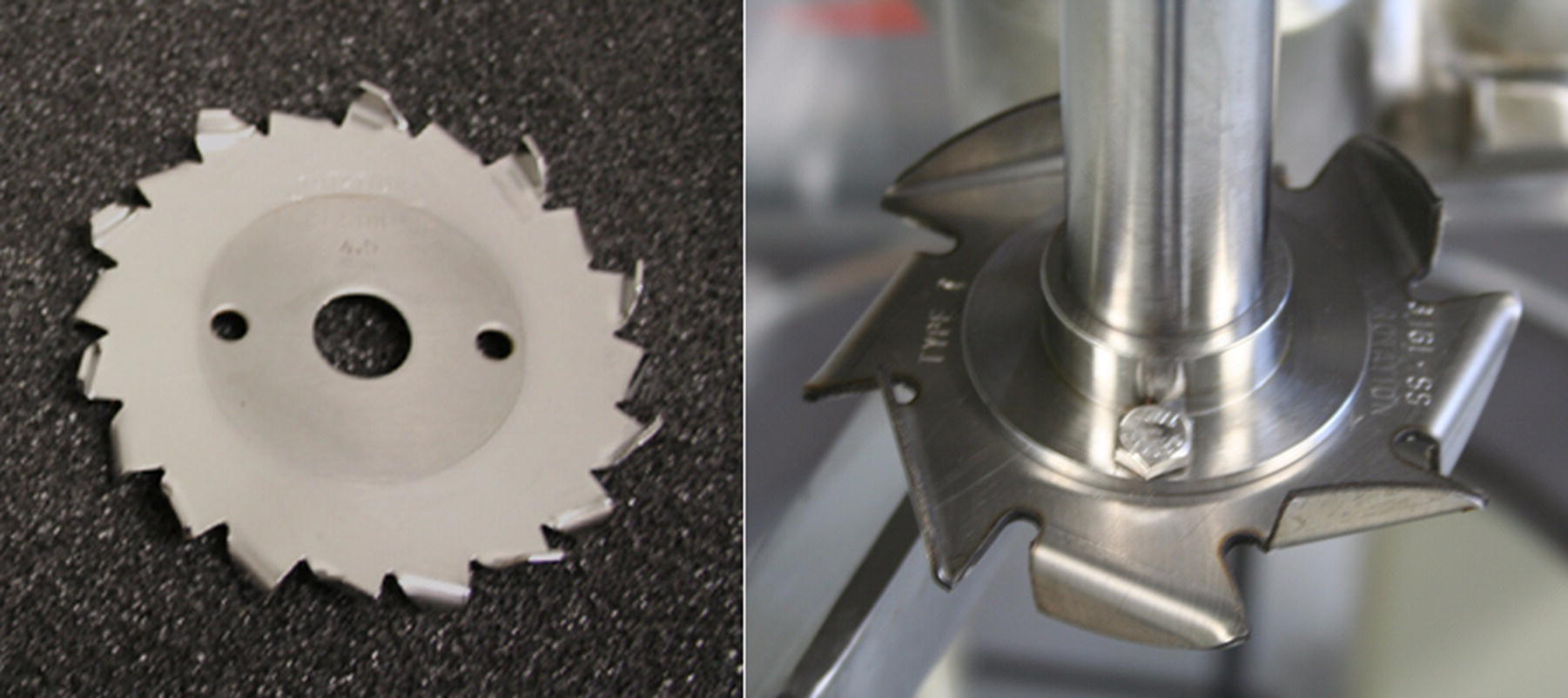
FIGURE 12.12 Two high‐speed disperser blades of different design. The blade on the right has a smaller number of teeth, but the teeth are larger than the standard Cowles design on the left. The blade with fewer, larger teeth will generate more flow than the Cowles blade but sacrifices some shear to achieve this.
Rotor–stator homogenizers provide a higher range of shear and energy dissipation than can be achieved by high‐speed dispersers. A typical rotor–stator homogenizer is shown in Figure 12.13. While the usual tip speeds (5–50 m/s) are not that much higher than high‐speed dispersers, much of the energy dissipation occurs within a small volume of liquid near the rotor and stator. This results in energy dissipation rates from 103 to 105 W/kg. This intense shear field results in very high shear stresses being transmitted to particles as they pass through the rotor–stator. Figure 12.14 shows the distribution of turbulent kinetic energy in a rotor–stator as predicted by CFD [15].
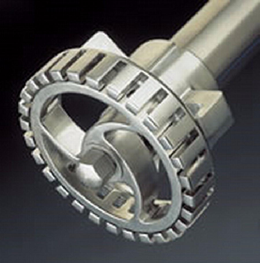
FIGURE 12.13 A typical rotor–stator homogenizer.

FIGURE 12.14 The distribution of turbulent kinetic energy in a rotor–stator as predicted by CFD.
Source: From Atiemo‐Obeng and Calabrese [15]. Copyright (2004) Wiley. Reprinted with permission of John Wiley & Sons, Inc.
There are many design variations of rotor–stator units, which alter the balance between pumping and shear. Rotor–stator homogenizers can be used in batch mode within a stirred tank or in‐line. In a stirred tank, it is best to provide an additional impeller to provide circulation and rely on the rotor–stator unit only to produce shear. In this way, the two effects can be decoupled, providing better control. This approach is essential when the fluid being mixed has significant yield stress. For yield stress fluids, multi‐shaft mixers can offer both close‐clearance impellers and rotor–stator homogenizers. While in‐line rotor–stator homogenizers provide some pumping, it is best to use a separate pump so that flow and shear can be controlled independently.
Tip speed is the most common approach for scaling up rotor–stator homogenizers. Given the many design variations that are available and the complexity of some of the designs, successful scale‐up depends on geometric similarity of the rotor–stator unit used at different scales. That being said, geometric similarity is not appropriate for the spacing between rotor–stator teeth. That gap must not be scaled up, but must remain constant across scales for a given process to ensure the same intensity of shear [15].
12.5 SCALE‐UP OF CHEMICAL REACTIONS
The scale‐up of processes involving chemical reactions presents a special set of challenges, particularly in nonhomogeneous systems or in semi‐batch reactions involving the controlled addition of reactive chemical reagents to a stirred vessel. Most chemical reactions are not 100% selective, that is to say that unwanted side reactions often accompany the main reaction. These reactions can reduce yield by consuming valuable starting materials, and the products of these side reactions can accumulate as contaminants that may be difficult or impossible to remove from the final product. These contaminants can also alter the crystal structure of some products, resulting in unexpected polymorphic crystal forms with poor solubility or other undesirable physical characteristics.
This can be a particularly vexing issue in an industry such as pharmaceutical manufacture, in which product quality is highly regulated and the presence of mere tenths of a percent of an unwanted impurity can result in an entire batch being rejected. Unfortunately, scaling up certain classes of reactions from a laboratory to commercial scale almost inevitably results in changes in selectivity, and often not for the better.
When a reaction is optimized in a laboratory setting, mixing is usually not an issue that comes into serious consideration, because laboratory stirrers provide very vigorous mixing and blend times in the one to two second range or less. However, upon scale‐up, the reaction will be run in a system in which blend time may be on the order of 30 seconds or longer (see Figure 12.6).
Consequently, as the reactive material is added to the reactor, it may swirl around in a highly concentrated plume for some time before it becomes dispersed throughout the reaction mixture. This localized zone of high concentration can cause an increase in side reactions that may not have been an issue in the lab, resulting in poor reaction selectivity and low batch quality. This is an extremely common problem in reaction scale‐up, and below we discuss some possible solutions. First, some examples of reactions that are affected by this phenomenon (so‐called mixing‐limited reactions) are in order.
12.5.1 Examples of Mixing‐Limited Reactions
Consider the so‐called Bourne [16] reaction, in which trimethoxybenzene (TMB) is treated with bromine to produce monobromotrimethoxybenzene (see Scheme 12.1).

SCHEME 12.1 The reaction between trimethoxybenzene and and bromine, and the consecutive competing reaction resulting in the formation of the di‐bromated side product.
This reaction suffers from a consecutive competing reaction, in which the mono‐Br product reacts with a second Br to form the di‐Br product. The rate of the primary reaction (k1) is about 1000× faster than that of the secondary reaction (k2), so one would expect little of the di‐Br to form. However, the rate of the secondary reaction is still fast enough that under typical mixing conditions, the mono‐Br product is not swept away from the site of the reaction quickly enough and undergoes the second reaction. Figure 12.15 shows that reaction selectivity can be somewhat improved by increasing the intensity of agitation.

FIGURE 12.15 The effect of mixing on the selectivity of the trimethoxybenzene (Bourne) reaction [16].
Another excellent example of the effect of mixing on reaction selectivity is the stereoselective enzymatic hydrolysis of a chiral organic ester (Scheme 12.2).
SCHEME 12.2 The stereoselective enzymatic hydrolysis of a chiral ester.
This is a biphasic reaction in which the enzyme is dissolved in the aqueous phase and preferentially hydrolyzes only one enantiomer of the chiral ester (an insoluble organic liquid) as it slowly enters the aqueous phase by diffusion. Base is added to maintain a constant pH as the acid product is formed.
Figure 12.16 shows the results of the reaction under conditions of good mixing and poor mixing. Note that under conditions of rapid mixing, the product purity is on the order of 99%, a result of the intrinsic selectivity of the enzyme, until the conversion reaches roughly 50%, at which point the preferred enantiomer is essentially all consumed and the enzyme begins to hydrolyze the other enantiomer. This results in reduced product purity at high conversions. However with poor mixing, the addition of the base causes nonselective chemical hydrolysis at the point of addition, resulting in lower product purity even at very low conversions.

FIGURE 12.16 The effect of mixing intensity on stereoselectivity of the enzymatic hydrolysis of a chiral carboxylate ester. y‐axis is enantiomeric excess (ee) of the product, a measure of enantiomeric purity. x‐axis is degree of enzymatic conversion.
A final example will illustrate the importance of mixing in heterogeneous reacting systems due to its effect on mass transfer. Consider the reaction between phenol and benzoyl chloride shown in Scheme 12.3.
SCHEME 12.3 The diffusion‐limited reaction between benzoyl chloride and phenol.
This reaction can be run in a biphasic system. The phenol is in aqueous solution, and the benzoyl chloride is a non‐water‐soluble organic liquid. In this process, the observed reaction rate is a function of both the intrinsic reaction kinetics and the rate at which the benzoyl chloride diffuses into the aqueous phase where it can react. As mixing speed increases, so does interfacial surface area (the dispersion droplets become smaller). This results in an observed increase in reaction rate because of the improved mass transfer, i.e. the faster rate of diffusion of the benzoyl chloride into the aqueous (see Figure 12.17).
FIGURE 12.17 The effect of mixing speed on the reaction between benzoyl chloride and an aqueous solution of phenol. As agitation rate increases, so does interfacial surface area and diffusion rate and consequently the observed reaction rate.
Source: Adapted from Atherton and Carpenter [17].
12.5.2 Identifying Mixing‐Limited Reactions
The types of reactions most likely to be affected by mixing upon scale‐up are highly rapid reactions, such as acid–base neutralizations. It is wise to try to identify any mixing‐dependent behavior of reactions in the laboratory prior to scale‐up to minimize surprises and failed batches. Sometimes it is simply a matter of running the chemistry in the laboratory under conditions of intense rapid mixing and of slow poor mixing. For example, for a controlled addition reaction, one could set up two side‐by‐side experiments. In one, the reagent is added slowly to a well‐mixed flask; in the other the reagent is added quickly to a flask with poor or no mixing. If there is a significant difference in product purity, then this system will likely experience issues at scale, and measures can be taken to try to minimize these effects prior to scale‐up.
A more theoretical approach is to calculate the Damkohler number for the reacting system. The Damkohler number (Da) is a dimensionless reaction time that represents the dependence of a given chemical reaction on mixing. Da is a function of reaction rate constant, reaction order, and reactant concentrations, but in simple terms, for semi‐batch reactions, Da is generally defined as a ratio between some characteristic mixing time scale and the time scale of the reaction.
The higher the value of Da, the more susceptible is the reaction to mixing effects. Figure 12.18 shows that for a very rapid reaction, such as an acid–base neutralization, the Damkohler number is much larger than 1, whereas for slow reactions, such as hydrolysis of an ester, the value of Da is much smaller than 1. The higher the value of Da, the more likely it is that the reaction could suffer changes in selectivity upon scale‐up.
FIGURE 12.18 An example of Damkohler number (Da) calculations for a rapid reaction and a slow reaction. The higher the value of Da, the more susceptible the reaction is to changes in selectivity due to mixing effects. The characteristic mixing time scale in this example is the blend time, here set to a typical value of 10 seconds.
12.5.3 Importance of Addition Point Design in Semi‐Batch Reactions
Now that we understand one of the main causes behind poor reaction selectivity upon scale‐up, we can examine some approaches to preventing it. In controlled addition reactions, selectivity can be improved by adding the reagent in such a way that it is dispersed and homogenized more rapidly. Therefore, rather than simply letting the reagent drip onto the surface of the batch or run down the side of the reactor, it should be injected at a zone of very high shear, such as right at the periphery of the rotating impeller using a delivery or “dip” tube.
For the best results, the tube must be properly sized (i.e. small enough diameter and high enough flow velocity) to prevent back mixing in the tube, which can lead to the same selectivity issues. Numerous setups are used to achieve rapid dispersion during chemical additions, some of which are shown in Figure 12.19. The perforated dispersion ring can be particularly useful in controlling pH by acid or base addition in biological or enzymatic systems that may be sensitive to high concentrations of these reagents. Some reactions have been significantly improved by spraying the reagent onto the surface of the batch by means of a “shower‐head”‐type arrangement.
FIGURE 12.19 Some systems for improving performance of semi‐batch or controlled addition reactions (from left to right: addition tube, dispersion ring, spray nozzle).
A number of other techniques are available for scaling up mixing‐sensitive reactions. One common approach is to install a static or mechanically agitated mixer in a forced recirculation loop. The reactive chemical reagent is then injected in a controlled fashion into the recirculation line just upstream of the in‐line mixer. This can speed dispersion and minimize the likelihood that a zone of very high concentration will exist in the vessel for any significant length of time. The static‐type mixers, of which there are many designs, are particularly useful because they are generally well characterized and have no moving parts that minimize maintenance.
12.6 CFD AND OTHER MODELING TECHNIQUES
One of the major tools for studying mixing and predicting mixing behavior in process equipment is CFD modeling. The advent of high‐speed personal computers has made CFD widely available, and it is finding use in many areas of technology, from plasma physics to the relatively simple liquid agitation we are concerned with here. Nonetheless, accurate modeling of fluid behavior requires the simultaneous calculation of huge numbers of equations, and even the simplest of problems consumes considerable CPU time.
Basically a mathematical model is constructed of the system of interest by dividing the fluid volume into hundreds of thousands or perhaps millions of contiguous cells (the model mesh; see, for example, Figure 12.20). The CFD software then tries to simultaneously solve the numerous momentum, velocity, force, heat transfer, and reaction mass balance equations associated with each of these cells in an attempt to converge on a single solution. When successful, these programs can accurately predict torque and mixing power requirements and can generate visual images or animations of fluid motion and circulation patterns that aid in identifying zones of high shear, stagnation, or other nonideal mixing behavior. Figure 12.14 shows an example of this type of image.
FIGURE 12.20 Showing the “wire mesh” for a portion of an A310 impeller for a CFD simulation of a stirred tank. The CFD mesh can consist of millions of three‐dimensional cells, usually with a finer grid size in the vicinity of the impeller where highest velocity and shear occur and coarser in the bulk fluid to save CPU time.
Several commercial software platforms are available for CFD modeling, but they are all quite expensive and require considerable expertise to properly code the model, create the mesh, and run the simulations. Needless to say, the success of the model depends on the accuracy of the rheological, chemical, and geometric data that is used to build it.
Some uncertainty is inevitable when conducting mixing experiments or modeling studies using computer simulations. For this reason most experts agree that for critical work, the CFD model should be validated by comparing predicted results with experimental measurements at least two different scales. In a typical scenario in which an industrial mixing system is to be designed based on the results of CFD modeling, the best results will be obtained if experiments are conducted first at some laboratory scale and then at a small pilot scale. CFD simulations of these two smaller‐scale operations would then be carried out, and once fine‐tuned to the point where predictions agree well with experiments, the model can be used for simulations to support the full‐scale design.
12.7 NOTATIONS
| A | racer concentration (outlet) |
| A0 | tracer concentration (inlet) |
| B | tank baffle width |
| C | impeller bottom clearance |
| D | impeller diameter |
| Da | Damkohler number |
| FCSTR | concentration ratio in CSTR |
| Gal | US Gal |
| hi | internal (process‐side) heat transfer coefficient |
| HP | horsepower |
| k | thermal conductivity |
| k′ | dimensionless Metzner–Otto constant |
| K | rheological consistency index |
| n | rheological behavior index |
| N | impeller rotational speed |
| NP | impeller power number |
| NQ | impeller flow number |
| NRe | impeller Reynolds number |
| NuL | Nusselt number |
| P | mixing power |
| Q | flow rate |
| St | tip speed |
| t | time |
| mean residence time | |
| T | tank diameter |
| TQ | torque applied to a mixer shaft |
| V | batch liquid volume |
| W | watt |
| Z | liquid height in batch vessel |
| α | ratio mean residence time/batch blend time |
| ε | rate of turbulent energy dissipation |
| ρ | density |
| η | Kolmogorov eddy length |
| ν | kinematic viscosity |
| shear rate | |
| μ | viscosity |
| τ | shear stress |
| τ0 | yield stress |
| θ | dimensionless residence time |
| Θ | batch blend time |
REFERENCES
- 1. Oldshue, J.Y. (1985). Current trends in mixer scale‐up techniques. In: Mixing of Liquids by Mechanical Agitation (ed. J.J. Ulbrecht and G.K. Patterson). New York: Gordon and Breach.
- 2. Uhl, V.W. and Von Essen, J.A. (1986). Scale‐up of fluid mixing equipment. In: Mixing: Theory and Practice Vol III (ed. V.W. Uhl and J.B. Gray), 155–167. Orlando, FL: Academic Press.
- 3. Johnstone, R.E. and Thring, M.W. (1957). Pilot Plants, Models, and Scale‐Up Methods. New York: McGraw Hill.
- 4. Kresta, S.M. and Brodkey, R.S. (2004). Turbulence in mixing applications. In: Handbook of Industrial Mixing (ed. E.L. Paul, V.A. Atiemo‐Obeng and S.M. Kresta). Hoboken, NJ: Wiley‐Interscience.
- 5. VisiMix (2006). Mixing Simulation Software, www.visimix.com
- 6. Hemrajani, R.R. and Tatterson, G.B. (2004). Mechanically stirred vessels. In: Handbook of Industrial Mixing (ed. E.L. Paul, V.A. Atiemo‐Obeng and S.M. Kresta). Hoboken, NJ: Wiley‐Interscience.
- 7. Rushton, J.H. et al. (1950). Power Characteristics of Mixing Impellers. Chemical Engineering Progress 46: 8 p395.
- 8. Grenville, R.K. and Nienow, A.W. (2004). Blending of miscible liquids. In: Handbook of Industrial Mixing (ed. E.L. Paul, V.A. Atiemo‐Obeng and S.M. Kresta). Hoboken, NJ: Wiley‐Interscience.
- 9. Penney, W.R. (1971). Recent trends in mixing equipment. Chem Eng 78 (7): 86.
- 10. Macosko, C.W. (1994). Rheology: Principles, Measurements, and Applications. New York: Wiley‐VCH.
- 11. Serth, R.W. (2007). Process Heat Transfer: Principles and Applications. Amsterdam: Elsevier.
- 12. Levenspiel, O. (1999). Chemical Reaction Engineering, 3e. Hoboken, NJ: Wiley.
- 13. Roussinova, V.T. and Kresta, S.M. (2008). Comparison of continuous blend time and residence time distribution models for a stirred tank. Industrial and Engineering Chemistry Research 47 (10): 3532–3529.
- 14. Etchells, A.W. and Meyer, C.F. (2004). Mixing in pipelines. In: Handbook of Industrial Mixing (ed. E.L. Paul, V.A. Atiemo‐Obeng and S.M. Kresta). Hoboken, NJ: Wiley‐Interscience.
- 15. Atiemo‐Obeng, V.A. and Calabrese, R.V. (2004). Rotor‐Stator mixing devices. In: Handbook of Industrial Mixing (ed. E.L. Paul, V.A. Atiemo‐Obeng and S.M. Kresta). Hoboken, NJ: Wiley‐Interscience.
- 16. Bourne, J. (2003). Mixing and the selectivity of chemical reactions. Organic Process Research & Development 7 (4): 471–508.
- 17. Atherton, J.H. and Carpenter, K.J. (1999). Process Development: Physicochemical Concepts. Oxford: Oxford University Press.