
10
CHARACTERIZATION AND FIRST PRINCIPLES PREDICTION OF API UNIT OPERATIONS
Joe Hannon
Scale‐up Systems Limited, Dublin, Ireland
10.1 INTRODUCTION
This chapter deals with how unit operations in API synthesis can be described, predicted, and scaled using classical chemical engineering principles. This allows design to be completed more quickly and with greater success than adopting a trial‐and‐error approach. Several common applications are worked through in detail for illustration. Examples and references to industry projects utilizing these concepts are included.
10.1.1 Rate Processes in API Unit Operations
Table 10.1 lists the rate processes involved in common unit operations in API synthesis. Characterization of each rate process is often feasible; the apparent complexity of unit operations arises from the combination of several rate processes in a single operation. In many cases, one rate process is limiting and dominates the others.
TABLE 10.1 Typical Incidence of Classical Chemical Engineering Rate Processes in Unit Operations
| Operation Rate Process | Reaction/Quench | Distillation | Extraction | Crystallization | Filtration | Drying |
| Chemical kinetics | ☑ | ☑ | ||||
| Mass transfer | ☑ | ☑ | ☑ | ☑ | ☑ | |
| Heat transfer | ☑ | ☑ | ☑ | ☑ | ☑ | |
| Addition | ☑ | ☑ | ☑ | ☑ | ☑ | ☑ |
| Removal | ☑ | ☑ | ☑ | ☑ | ☑ |
Other chapters in this book also address several of these rate processes and operations, including “REACTION KINETICS AND CHARACTERIZATION,” “ANALYTICAL METHODS FOR MASS BALANCE AND REACTION KINETIC ANALYSES,” “DESIGN OF DISTILLATION AND EXTRACTION OPERATIONS,” “DESIGN AND SCALE‐UP OF PHARMACEUTICAL CRYSTALLIZATIONS,” “DESIGN OF FILTRATION AND DRYING OPERATIONS,” “KILO LAB AND PILOT PLANT MANUFACTURING,” “QUALITY BY DESIGN APPROACHES FOR API,” and “QbD CASE STUDY: API CASE STUDY.”
10.1.2 Scale Dependence and Scale Independence
The intrinsic rate of a chemical reaction is independent of scale; in other words, if the reaction could be conducted without limitation by any other rate process, it would run at the same rate (per unit volume) at all scales; the reaction time, starting from the same initial composition and held at the same temperature, would be the same at all scales. This is true for reactions whose kinetics are slow compared with other rate processes. The choice of solvent, reagents, and/or catalyst combination for reactions has been largely the domain of development chemists, and these variables are taken here to be fixed already; in any case, those effects, including reagent solubility, are also independent of scale.
All other rate processes listed in Table 10.1 are scale dependent. For example, the rate of heat transfer depends strongly on the ratio of surface area to volume, which reduces on scale‐up. This means that heat removal on scale will be slower than in the laboratory, unless specific measures are taken to provide additional surface area or an increased temperature driving force. Therefore the time required to heat or cool a batch of material tends to increase on scale. Similarly, the rate of mass (or phase) transfer is scale dependent; the agitation conditions inside the vessel determine the time required to reach equilibrium between the phases; it is easier to make this time short in the lab than on scale.
The rates of addition and removal of material also change with scale, normally taking longer at larger scales. For example, the rate of disengagement of gas evolved from a reaction depends again on the surface‐area‐to‐volume ratio, so reactions such as decarboxylation have to be conducted more slowly on scale to avoid partial loss of the reactor contents due to swelling of the batch.
The impact of scale dependence is to lengthen processing times on scale, reducing productivity somewhat but more importantly potentially allowing additional phenomena to occur that were not observed to the same extent in the laboratory, such as impurity‐forming reactions, product degradation, catalyst poisoning or deactivation, unwanted crystal forms, nucleation, agglomeration, or breakage. Fortunately, each of the rate processes that contribute to such problems can be characterized or estimated using classical chemical engineering methods, allowing scale‐up problems to be anticipated and resolved in advance or at least resolved quickly once they occur.
10.1.3 Scale‐Up and Achievement of Similarity
Unit operations need to produce similar results and a similar quality product at each scale; historically the pharmaceutical industry has demonstrated this through process validation at each facility and operation thereafter with rigid limits on process parameters. Recent regulatory guidance [1] encourages adoption of “quality by design” (QbD) and development of a “design space” in which the process may operate, with flexibility to move operating conditions around in this space without needing to obtain additional regulatory approval. The design space is proposed by the applicant and is intended to be applicable to the process at any scale. This implies a greater investment in developing process understanding during the development phase, balanced by flexibility, a reduced regulatory burden, and opportunities for continuous improvement once the process is in full‐scale manufacturing.
There is some debate about how best to apply these principles while also satisfying business, process safety, and environmental requirements, and the underlying benefit of improved process understanding is underlined in this chapter. The operating window in which acceptable or similar results are obtained can be determined, demonstrated, and justified in terms of the chemical engineering rate processes involved in unit operations. For example, the design space for a chemical reaction whose intrinsic kinetics have been shown to be slow (compared with other rate processes involved) can be demonstrated to be scale independent, giving a flexible operating window that can be used at any scale. On the other hand, where specific equipment performance requirements exist, these can be framed in terms of the chemical engineering “rate constants” or time constants required by the process.
In the next section, we will see that these rate constants arise naturally in the chemical engineering rate equations, which provide a first principles basis for defining a scale‐independent design space. The application of this approach is illustrated for several common types of chemical reaction, and the same general principles and methods apply to other API synthesis operations. Examining the rate equations also leads to familiar scale‐up rules.
10.1.4 Characterization of Reaction Systems
Guidance specific to certain classes of reaction is given below, but to avoid repetition for each class, the following general guidelines on reaction characterization are provided here. Guidelines on equipment characterization are given toward the end of the chapter.
Assuming that the solvent and reagents/catalyst have been selected, reactions may be characterized by a sequence of initial screening experiments to identify scale‐dependent physical rate process limitations, followed by a more detailed kinetics study if necessary.
In all experiments aimed at characterizing a reaction, progress should be followed by either taking multiple samples or using an in situ analytical technique, not by relying on a single endpoint sample. If composition is analyzed using HPLC, determination of response factors will become more important as characterization proceeds. Other possibilities include infrared (IR), ultraviolet (UV), and Raman spectroscopy or heat flow (Qr).
Samples should be analyzed to indicate both reaction progress (e.g. product level, conversion, or current yield) and product quality (e.g. impurity level). If either of these variables is sensitive to physical rates (e.g. agitation), the reaction is not limited by chemical kinetics, at least under typical processing conditions. There may be some scope to reduce the rates of the chemical reactions (relative to mixing) by operating at, e.g. lower concentrations and/or temperatures; otherwise, if the process persists in its current form, the focus of characterization should be the physical capabilities of lab and larger‐scale equipment (see Section 10.6).
Under conditions where there is no effect of physical rate processes, a kinetics study may follow in which temperature, equivalents, and/or other case‐specific variables affecting the scale‐independent chemical rates are varied experimentally. The choice of conditions and the sampling program for these experiments should be informed by the results of the previous experiments and an initial kinetic model [2], and in any event, multiple samples should be taken again to capture when the reactions are occurring as well as the final result.
Where possible, the parameters in Eq. (10.3) such as rate constant and activation energy should be fitted using a kinetic model to reliable results of experiments. Model development in this manner tends to be iterative, and the proposed reaction scheme may change a number of times before the model fits the data to an acceptable degree. Chemical knowledge that certain intermediate species is unlikely to exist for long may allow the rate constants of certain reactions to be set arbitrarily high so that the remaining parameters can be fitted with greater confidence. Model development should take place at the same time as experimentation and the design of remaining experiments may change as a result of indications from the model.
It is difficult to overemphasize the importance of conducting a few well‐designed, well‐monitored experiments versus a large set of experiments with scant data recording. Isothermal experiments are preferred, though not absolutely necessary as long as the temperature versus time is recorded during the heat‐up and the location of “time zero” is clear. HPLC remains the most powerful method to follow product and impurity levels, and it is preferable to convert directly from HPLC area to moles rather than HPLC area percent. When starting materials are sufficiently pure, enough peaks are captured by HPLC, several response factors are known, and (preferably) an internal standard is also used, assumptions about the reaction scheme proposal can be checked directly using HPLC area. This can reveal the existence of undetected intermediates or by‐products and allow the reaction scheme to be revised accordingly. An excellent illustration of the procedure is available [3].
At the end of this phase, such a model may be used to find optimum conditions inside or outside the experimental region and to assist with definition of a scale‐independent design space. Some excellent examples of the success of this approach are available [4–8]. Further experimentation should be focused on model verification, especially at the most forcing conditions over which it may be used.
10.2 BATCH PROCESSES WITH HOMOGENEOUS REACTIONS
Figure 10.1 shows a “process scheme” for a batch reaction. This consists of a simple representation of the (i) phases and (ii) rates involved in the operation. The phase names and components initially present are indicated together with the rate processes. More or less detail may be added to such a schematic as required, and this representation will be used below to introduce other operations.
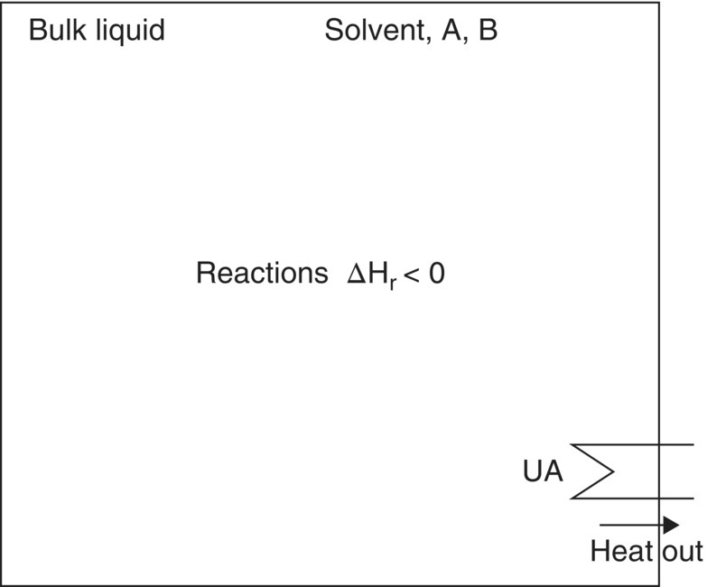
FIGURE 10.1 Process scheme for batch homogeneous reaction.
10.2.1 Rate Equations
If, for example, the reaction involved is simply A + B → P, the rate equations for this system may be written as follows. The rate of change of concentration of A or B is
where the rate expression on the right‐hand side is of this or similar form:
and the kinetic rate constant follows the Arrhenius relationship
More generally than (Eq. 10.1), and when several reactions are occurring in the same mixture, the rate of change of concentration of any species in the mixture is given by
From Eqs. (10.1) to (10.4), the rate constant depends on temperature, and the rates of reaction depend on concentrations. This is the chemical engineering basis for the classical approach by chemists to study temperature and “equivalents” as two of the primary variables affecting the outcome of a reaction. In the above example, with 1 mol of A reacting with 1 mol of B, 1 equiv. of A would mean 1 mol of A/mol of B, 2 equiv. of A would be 2 mol of A/mol of B, etc.
Integrating Eq. (10.4) in time, the final outcome (composition) of reaction will depend on the concentrations and temperature profiles followed during reaction and the time allowed for reaction. Temperature is often (but not always) held constant or nearly constant, in which case final concentrations at completion depend only on initial concentrations and initial temperature. Example Problem 10.4 follows this behavior.
Temperature is an important influence and can change the relative rates of the reactions, depending on their activation energies. From a safety standpoint, temperature must be controlled to avoid thermal runaway, and the batch reactor is not ideal for this purpose. The rate of change of reactor temperature is given by

In which the log mean temperature difference is

The approximation on the right of Eq. (10.6) applies when the heat transfer fluid flow rate is high, i.e. the heat transfer fluid temperature is almost constant between the jacket inlet and outlet.
The rate of heat evolution summed over all chemical reactions in the mixture is
Note that heat of reaction in Eq. (10.7) is the heat released per mole of reactant consumed when the stoichiometric coefficient of that reactant is 1 and is negative when the reaction is exothermic. Equation (10.5) shows that temperature can be controlled by balancing scale‐dependent heat removal with scale‐independent chemical kinetics. The former can be enhanced by increasing the surface area and/or increasing the temperature driving force, normally reducing the jacket inlet temperature. These measures can allow the reaction to run at the same temperature and concentration on scale, in the same reaction time as in the laboratory. There is an upper limit on the scale at which this will be feasible. On the other hand, reaction rate can be reduced to balance reduced heat removal by operating at lower concentration or lower temperature; the former reduces productivity; the latter could change the balance between desired and undesired reactions, lengthens reaction times, and also reduces the available temperature driving force for cooling.
For the common case where the temperature is held constant during reaction and the initial concentrations are the same at each scale, Eq. (10.5) with the left‐hand side set to zero leads to the scale‐up basis
Equations (10.4) and (10.8) taken together indicate that for scaling batch homogeneous reactions that are limited by chemical kinetics, a scale‐independent design space can be expressed using temperature and equivalents as factors, as long as there is sufficient assurance that adequate heat transfer to maintain temperature control will be available at all scales. The latter condition amounts to a statement about the equipment capability at each location, specifically the heat removal capacity (in W/l) of the equipment operating at the required temperature.
All of the above effects can be calculated using mechanistic models in which Eqs. (10.2)–(10.7) are solved by integration in time. In practice, batch homogeneous reactions may not be allowed to run to completion, because stopping the reaction earlier produces higher yield (yield peaks during the batch) and less impurity than waiting until the end. Similarly, batch homogeneous reactions may be run using temperature profiles, e.g. charge at low temperature, heat to reaction temperature, then hold, and possibly heat again. In these cases, the temperature profile followed by the reaction may be scale dependent for the reasons given above, with, e.g. longer heating ramps on scale; this will impact the relative rates of the reactions and could affect quality as well as rate.
If Eq. (10.3) is known for each reaction, these effects can be predicted easily, and operating conditions can be optimized to a high degree as shown in Example Problem 10.4; good examples of this approach covering a variety of reaction types are available [9–13].
10.2.2 Characterization Tests for Batch Homogeneous Reactions
The general guidelines described in Introduction should be followed with regard to experimental design.
The reaction should first be run in 2–3 otherwise identical (replicate) experiments in which stirrer speed is varied between 200 and 1000 rpm; four or more samples should be taken, biased toward the beginning of the reaction, e.g. after 10, 30, 60 minutes, and at the end.
Under conditions where there is no effect of physical rate processes, a kinetics study may follow in which temperature and equivalents are varied experimentally and the parameters in Eq. (10.3) fitted.
If agitation conditions affected the result of the initial screening experiments, the result of the reaction is influenced by the rate of mixing or more specifically the rate of bulk blending of the vessel contents, known as “macromixing.” This is unusual for a batch homogeneous reaction, but if it occurs, the scale‐dependent macromixing time constant will be important as the outcome of reaction is influenced by this characteristic and not just chemical kinetics; see the section below on equipment characterization. A reaction such as this might be better run in fed‐batch mode, with the fed reagent maintained at a low concentration. Alternatively, there may be some scope to reduce the rates of the chemical reactions (relative to mixing) by operating at lower concentrations and/or temperatures.
10.2.3 Achieving Similarity on Scale‐Up
Achieving similarity on scale‐up relies on having characterized both the reaction and the intended scale‐up facility. Equations (10.2)–(10.7) provide the basis for a scale‐independent design space.
When kinetics are rate limiting, other than agitation that is necessary to promote heat transfer, no particular additional agitation requirement exists for homogeneous reactions. As noted above, there may be an optimum temperature profile to adopt during reaction and/or an optimum time at which to stop the reaction. These may be determined from a kinetic model, as in Example Problem 10.4. A scale‐independent design space may include factors such as equivalents, temperature, and reaction time.
When mixing is rate limiting, unusual for batch homogeneous reactions, agitation influences the outcome, and similar macromixing time constants will be required at each scale; if the process persists in this form, the macromixing time constant should be a factor in design space definition.
10.3 MULTIPHASE BATCH PROCESSES WITH REACTIONS
Figure 10.2 shows a schematic of a multiphase batch reaction, in this case a hydrogenation.

FIGURE 10.2 Process scheme for a hydrogenation, an example of batch multiphase reaction.
These reactions are also referred to as “heterogeneous,” “biphasic,” or “slurry phase.” Figure 10.2 shows the main liquid phase initially containing substrate, another phase (the headspace) containing reagent (hydrogen), reaction in the liquid phase between substrate and dissolving reagent (hydrogen) and removal of heat. (In Figure 10.2, the solid catalyst phase that is normally present for hydrogenation is omitted, and the catalyst particles are assumed to follow the liquid. The headspace is continuously replenished with hydrogen as reaction proceeds.)
10.3.1 Rate Equations
Although relatively complex at first sight, this multiphase, chemically reacting, time‐dependent problem can be broken into classical chemical engineering elements and rate processes just like the batch homogeneous reaction above. The rate equation for chemical species concentration in the liquid phase is given by combination of chemical kinetics with the film theory of scale‐dependent mass transfer:
Only the equations for components that transfer between phases contain the second term; for dissolving gases, solubility is given by Henry's law:
In other heterogeneous reactions, the solubility expression differs; for liquid–liquid (aqueous–organic) systems,
where Si is the partition coefficient for component i between the phases. For solid–liquid systems,
where f() is a function determined from phase equilibrium fundamentals and/or by experimental measurement (e.g. using NRTL equations or similar).
When the transferring component is a solvent (e.g. in a reactive distillation or solvent swap), the equilibrium is described using the Antoine or similar vapor pressure equation [14].
Examination of Eq. (10.9) indicates that when chemical kinetics are slow relative to mass transfer, the concentration of hydrogen (or any dissolving, reacting solute) will tend to saturation with modest kLa values. On the other hand, if in Eq. (10.9), the kinetics of reactions consuming hydrogen are rapid compared to mass transfer, the concentration of hydrogen will tend toward zero during reaction. These two extremes of behavior change the outcome of reaction; slow mass transfer extends reaction time, may lead to increased impurities, and can cause reaction to stall. The outcome of a batch multiphase reaction at constant temperature therefore depends on temperature, concentration, equivalents (including catalyst loading), pressure (if the solute is in the gas phase), and potentially kLa.
In reactions with three phases present, such as the additional solid catalyst phase in hydrogenation, that phase should be dispersed, and its surface area made available for mass transfer in a similar way to the gas phase in the present example. Complete suspension of a solid phase is usually sufficient to prevent mass transfer to or from that phase being rate limiting; when the solid particles have the same characteristics at both scales, complete suspension is approximately equivalent to maintaining constant kLa for those particles (see the Section 10.6).
For multiphase reactions, the rate equation for solution phase temperature is
Equation (10.13) contains one additional term compared with Eq. (10.5) to account for any heat effect associated with mass transfer of dissolving material between phases; this effect is often negligible but can be significant when solvent is vaporized (in distillation) or when a large quantity of solute is transferred quickly (e.g. when crystals come out of solution suddenly). The heat flow signature from the chemical reactions will be determined by kinetics when mass transfer is rapid and by mass transfer when kinetics are rapid. Neglecting the final term in Eq. (10.13), the scale‐up relationship for maintaining constant temperature when kinetics limit is identical to the corresponding equation for homogeneous reactions:
Equation (10.14) when applied to pressure reactions assumes constant pressure, i.e. constant solubility. The scale‐up relationship when kinetics are rapid relative to mass transfer can be obtained by noting that in this case, the rate of dissolution of the limiting solute dominates the rates of the main reactions:
Substituting Eq. (10.15) into Eq. (10.13) leads to
The above result may also be obtained by writing Eq. (10.13) in dimensionless form using t* = kLa·t and T* = T/T0, neglecting the last term and substituting Eq. (10.15) for Qr:
The second term on the right‐hand side is constant when pressure and initial temperature are fixed, and when the left‐hand side is set equal to zero (constant temperature), Eq. (10.16) is obtained.
Equations (10.16) and (10.17) indicate that when the solution concentration of solute is close to zero, the required rate of heat removal is directly proportional to the rate of mass transfer, i.e. higher kLa implies the need for greater heat removal.
An additional constraint exists for pressure reactions, such as hydrogenation, which cannot be taken for granted in practice. The ability to maintain a desired or constant pressure in the headspace depends on the balance between supply of fresh gas to the headspace and removal of gas by mass transfer:
Equation (10.18) shows that rapid mass transfer may cause the headspace pressure to reduce, while a temperature rise may cause it to increase. To maintain a constant pressure on scale‐up requires adequate temperature control and adequate gas supply:
The right‐hand side of Eq. (10.19) requires knowledge of the solution concentration of the dissolved gas. A conservative estimate may be made by setting the dissolved concentration to zero, leading to
A crude estimate of the required flow rate to maintain constant pressure may also be made from the number of moles of gas required for reaction and the intended reaction time, i.e.
Similar to homogeneous batch reactions, Eqs. (10.9)–(10.13) and (10.18) can be easily incorporated into dynamic mechanistic models for multiphase reactions and the unknown parameters (e.g. rate constants, activation energies) regressed against experimental data. The effects of changing concentrations and equivalents (including catalyst loading), temperatures, and pressures and the effects of mass transfer, heat transfer, and gas supply limitations can then be predicted. In many hydrogenations, for example, neither pressure nor temperature is maintained constant, and the profiles they follow may be scale dependent; even the sequencing of nitrogen and hydrogen purges before reaction can affect the result. The impact of these changes can be predicted using classical chemical engineering rate equations with appropriate reaction and equipment characterization. Example Problems 10.1 and 10.2 illustrate this approach.
10.3.2 Characterization Tests for Multiphase Reactions
The general guidelines described in Introduction should be followed with regard to experimental design.
For gas–liquid, gas–liquid–solid, liquid–liquid, and liquid–liquid–solid systems, the reaction should first be run in 2–3 otherwise identical (replicate) experiments in which stirrer speed is varied between 200 and 1000 rpm; 4 or more samples of the reacting phase should be taken during reaction, biased toward the beginning of the reaction, e.g. after 10, 30, 60 minutes, and at the end. With some reactions, additional profiling may be possible by following variables such as hydrogen uptake, pressure, and both pot and jacket temperature. The purpose of changing stirrer speed is to change the mass transfer contact area between the phases. In each of these experiments, any solids present should be well suspended.
To check for mass transfer limitation due to dissolving solids, experiments should be run at an impeller speed, which guarantees suspension, but either the particle size or the mass of solid reagent should be varied.
Under conditions where there is no effect of physical rate processes, a kinetics study may follow in which any of temperature, equivalents, pressure, catalyst loading, and/or other case‐specific variables affecting the scale‐independent chemical rates are varied experimentally.
If agitation conditions affected the result of the initial screening experiments, the outcome of the reaction is influenced by the rate of mass transfer. This is frequently the case for heterogeneous reactions, and characterization of the scale‐dependent equipment characteristics will be important. There may be some scope to reduce the rates of the chemical reactions (relative to mixing) by operating at lower concentrations, pressures, catalyst loadings, and/or temperatures, but this will also reduce volumetric productivity.
10.3.3 Achieving Similarity on Scale‐Up
For batch multiphase reactions, achieving similarity on scale‐up relies on having characterized both the reaction and the intended scale‐up facility. Equations (10.9)–(10.13) and (10.18) provide the basis for a scale‐independent design space.
When kinetics are slow (relative to mass transfer), adequate agitation is necessary to create a dispersion and to promote heat transfer; adequate gas supply is required for pressure reactions. Justifying the scale independence of the design space in this case reduces to demonstrating that pressure and temperature can be maintained in the same range on scale as in the laboratory and that agitation is sufficient to disperse the phases.
When kinetics are fast, kLa should be included explicitly to make the design space scale independent.
For hydrogenations and other catalyzed pressure reactions, a design space could therefore contain concentrations, equivalents, temperature, pressure, catalyst loading, and time as factors; when kinetics are fast, kLa should also be a factor.
As noted above, there may be an optimum temperature or pressure profile to adopt during the reaction and/or an optimum time at which to stop the reaction. These may be determined from a kinetic model, as used in the example described below [15]. Many examples of kinetic modeling of multiphase reactions are available, including a methanethiol reaction [16] and for other hydrogenations [17].
When kinetic models are used in reverse, to work backward from a desired end result to determine the possible operating conditions (or factors) that would produce this result, multiple acceptable combinations of factor settings may be found. For example, very poor mass transfer (low kLa) can be partially compensated for by operating at higher pressure [18]; the effects of low kLa may also be partially mitigated by operating at lower concentrations of starting materials or catalyst. These combinations may be difficult to express in a design space definition but can be found easily using a mechanistic model and justified if the model has been properly verified against experimental data. This has led to discussion of the use of models to more flexibly capture the definition of a design space and verify that a given set of operating conditions lie within it [19].

FIGURE 10.3 Lab results (discrete points) of this hydrogenation (reduction of a nitro group, Example Problem 10.1) indicated a six hour reaction time. Modeling (continuous curves) and vessel characterization revealed this was due to severe gas–liquid mass transport limitations (kLa) in the lab equipment and that the process could perform much better.
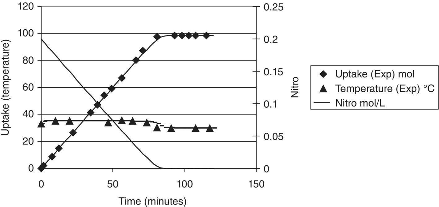
FIGURE 10.4 A reaction time of 1.5 hours was predicted (curves) and achieved (symbols) in the pilot plant for the same reaction as in Figure 10.3 (Example Problem 10.1). The mass transfer characteristics of the pilot plant reactor were superior to those of the lab reactor.
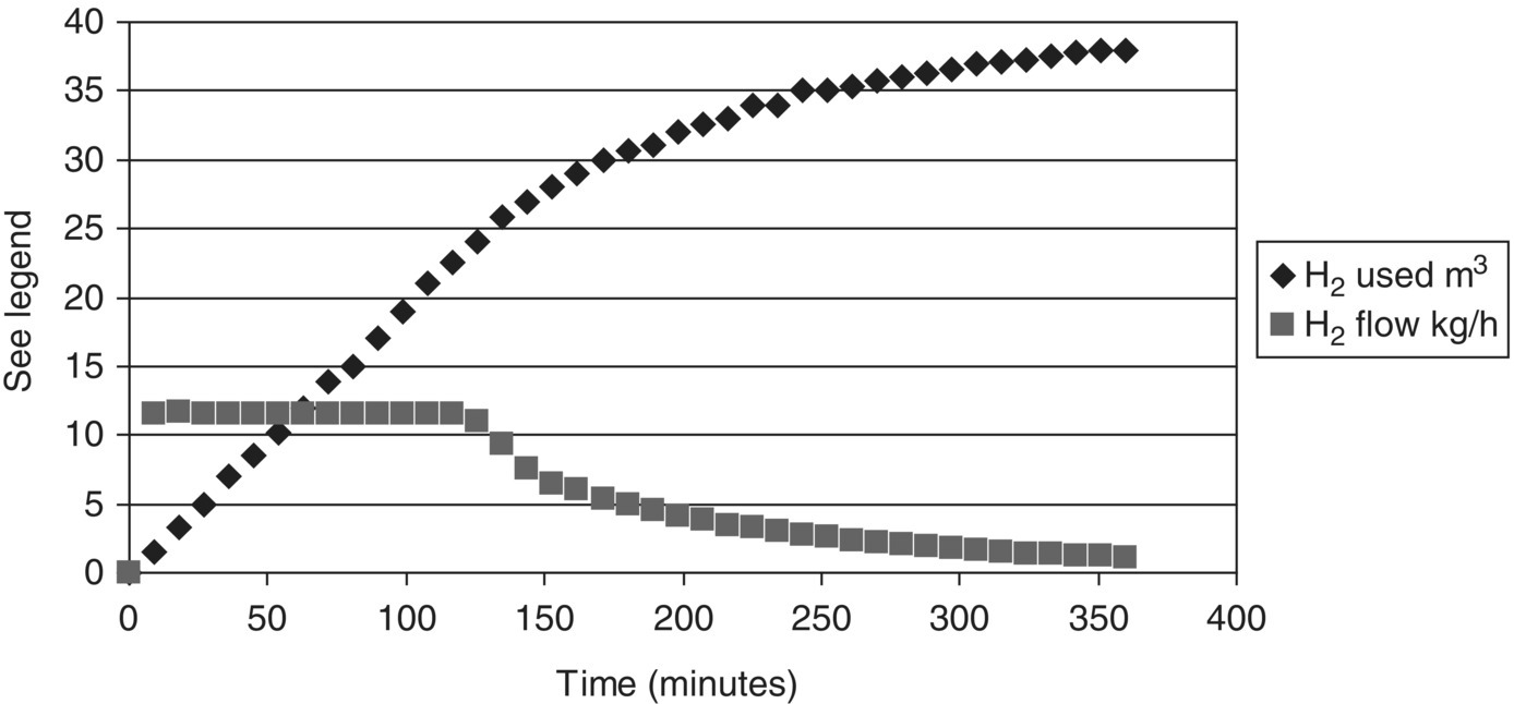
FIGURE 10.5 On scale‐up of another hydrogenation (Example Problem 10.2), reaction times extended to over six hours, due to the appearance of a bimodal particle size distribution in the solid substrate, with about 50% of the solids mass having a much larger particle size; this reduces the rate of reaction, especially once the smaller solids have dissolved.
10.4 FED‐BATCH PROCESSES WITH REACTIONS
Figure 10.6 shows a process scheme for a homogeneous fed‐batch reaction.
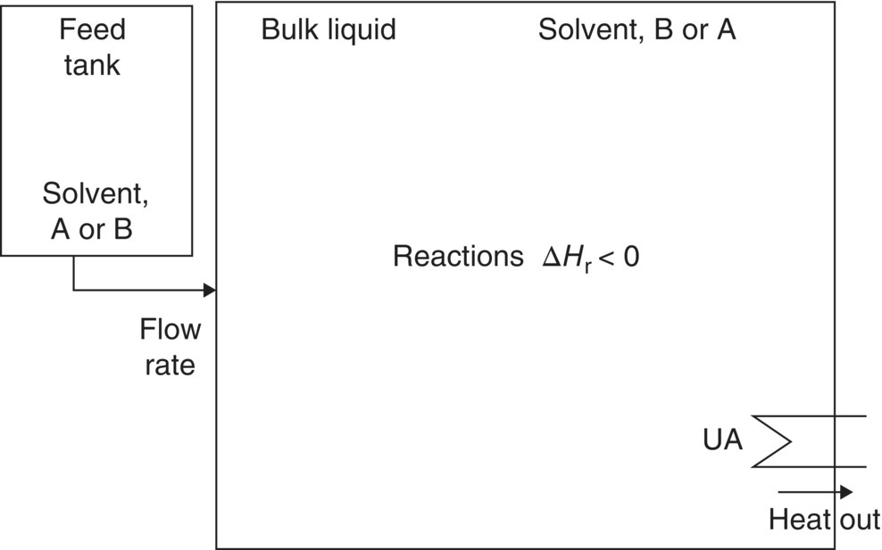
FIGURE 10.6 Process scheme for a homogeneous fed batch reaction system.
These operations are common both in the laboratory and on scale and are also known as “exothermic additions” or “semi‐batch reactions.” Figure 10.6 shows the main reaction liquid phase initially containing solvent and one or more reactants, with another reactant initially in the feed tank. Liquid is added from the feed tank, reaction begins, and the resulting heat is removed.
10.4.1 Rate Equations
The rate of change of concentration of each species in a homogeneous fed‐batch reaction is
Compared with Eq. (10.4), the additional term on the right‐hand side represents addition of feed and the accompanying dilution effect.
When the kinetic rates of the reactions are slow compared with the rate of addition, reaction takes place after the addition, and the result is very similar to a homogeneous batch reaction, described above. When the kinetic rates are comparable with the addition rate, a significant amount of reaction occurs during the feed, which normally changes the outcome of reaction compared with the batch case. This is because the concentration of the fed reactant remains low during the addition.
When the kinetic rates are much faster than the addition rate, the concentration of the fed reactant tends to zero, and in this case the reaction is highly localized around the feed region. Equation (10.22) in this case no longer fully describes the rates of change, and a more detailed analysis involving phenomena known as mesomixing and micromixing is required [20, 21] for an accurate mathematical description. A process scheme for this situation is shown in Figure 10.7, with the notable addition of a “feed zone” or reaction zone in which most of the reaction takes place. The size of the feed zone and its composition are determined by micromixing and mesomixing rates. The outcome of the reaction is predominantly determined by these scale‐dependent rates rather than by chemical kinetics.
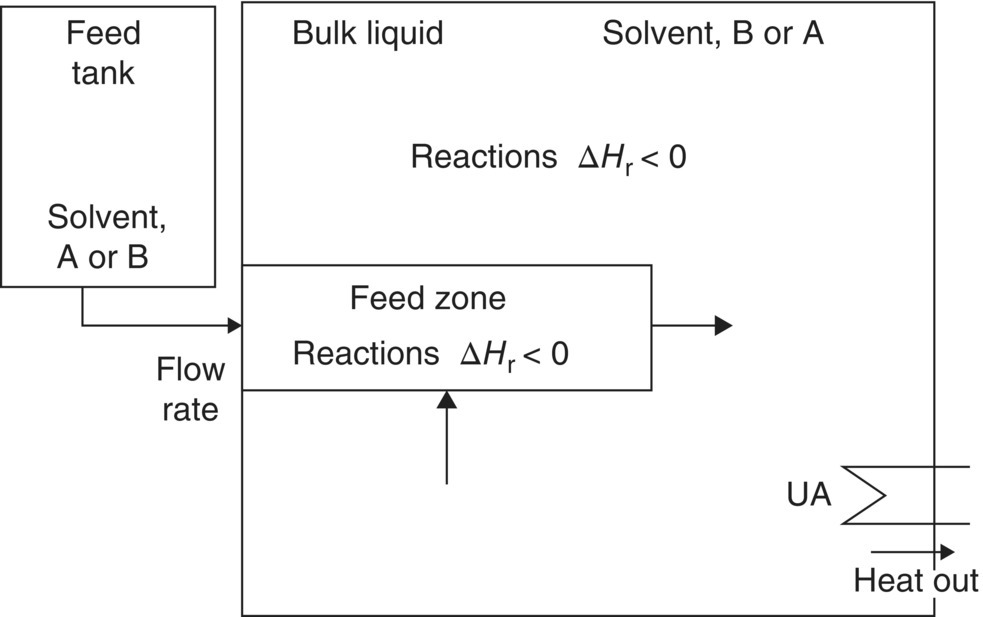
FIGURE 10.7 Process scheme required for a fed batch reaction with rapid chemical kinetics.
The rates of mesomixing and micromixing can be thought of as somewhat analogous to the rate of mass transfer between two phases, which arises with multiphase systems as described above; for this reason, fed‐batch reactions with rapid chemical kinetics are often referred to as “pseudo‐homogeneous,” implying that the feed zone is like a separate phase.
The characteristics in Figure 10.7 arise in a significant fraction of applications, as reactions are often deliberately engineered to run with fast kinetics (e.g. by operating at high concentration, catalyst loading, and temperatures) because the heat output from such systems can then be halted in the event of a cooling failure by stopping the addition. Reactions such as these are also known as “feed controlled” and “dosing controlled.” The existence of the feed zone does not necessarily change the outcome of the reaction significantly; this only occurs if the reaction scheme and kinetics are such that the concentration and temperature “hotspot” that exists in this zone causes the reactions to follow a different path compared with what they would follow if diluted fully throughout the bulk of the vessel. In a significant minority of cases, the feed zone has a major bearing on product quality and yield. Appropriate characterization experiments as described below can be used to determine whether a given reaction is subject to these effects.
Considering Eq. (10.22), when reaction kinetics are slow, such that all or almost all of the reaction takes place after the addition is complete, the solution tends toward that for a batch reaction with the same volume, as described by Eq. (10.4). Integrating Eq. (10.22) in time, the final outcome (composition) of the reaction will then depend on the concentrations and temperature profiles followed during the reaction and the time allowed for the reaction. Temperature is often (but not always) held constant or nearly constant, so final concentrations at completion depend only on initial concentrations and initial temperature. Example Problem 10.4 follows this behavior.
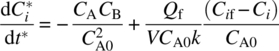
When a significant amount, but not all, of the reaction occurs during feeding, this indicates that some of the chemical kinetic rates are comparable with the addition rate. Equation (10.22) is more informative for this case when examined in dimensionless form; for a second‐order reaction between A and B, using ![]() =Ci/CA0 and t* = kCA0·t, the rate equation for the dimensionless A or B concentration is, from Eq. (10.22),
=Ci/CA0 and t* = kCA0·t, the rate equation for the dimensionless A or B concentration is, from Eq. (10.22),
Or, equivalently,
Defining the initial volume ratio of bulk solution to feed solution as
and noting that feed time is given by
then, at the start of the addition,1
Substituting Eq. (10.27) into Eq. (10.24) leads to
Equation (10.28) shows that the outcome (or dimensionless concentration profile) of fed‐batch reaction when a significant amount of reaction occurs during the addition depends on the initial concentrations in the bulk and feed vessels, the rate constant (temperature dependent), the addition time, and also the volume ratio of the reagents. This latter point is important as the volume ratio is independent of the number of equivalents, i.e. reactions run at the same equivalents, temperature, and addition time may produce different results when the volume ratios mixed are different.
Apart from volume ratio, a further degree of freedom exists in fed‐batch reactions that is not present in the batch case: the order of addition; when the order of addition is reversed, this can radically change the solution concentrations compared with the forward addition. Reverse addition is worth considering and testing when feasible and safe. From a quality point of view, order of addition should follow from the reaction scheme (expressed in Eq. (10.4) using the stoichiometric matrix νij). For example, in the following case, to maximize product it is more favorable to add A to B:
- A + B → product
- A + product → impurity
In the next case, it is more favorable to add B to A:
- A + B → product
- B + product → impurity
When essentially the entire reaction occurs during the addition, Eqs. (10.22) and (10.28) are no longer directly applicable, as the reaction zone will be localized and some reactions will run to completion before the feed has been diluted into the bulk contents. In this case, the dominant effect on the composition of the reaction mixture is the rate of localized mixing near the addition point, a physical phenomenon somewhat analogous to mass transfer in the multiphase example above. The degree to which the reaction exhibits this characteristic may depend on the order of addition. The final outcome of this type of reaction will depend on the time constants for mesomixing or micromixing, whichever is slower and therefore rate determining; these influence the size and residence time of the feed zone, which in turn determines how much of the chemistry takes place in the concentration and temperature hotspot created by the feed. Both meso‐ and micromixing time constants are affected by the addition rate, the addition location, the diameter of the addition nozzle, the agitator configuration, and the agitator rotational speed [14]. Factors directly affecting the intrinsic kinetics have less influence in this scenario, such as reaction temperature.
The rate of change of temperature in fed‐batch reaction systems is given by
Compared with Eq. (10.5) for batch reactions, the two additional terms on the right‐hand side represent contribution of sensible heat by the fed material (e.g. when warmer than the bulk) and any associated thermodynamic heat of mixing that also accompanies the addition. The heat flow signature from the chemical reactions will be determined by kinetics (kinetically controlled) when reaction occurs after the addition, by the rate of addition when the reactions occur entirely during the addition, and by both kinetics and the rate of addition when a significant amount of reaction, but not all, occurs during the addition.
From Eq. (10.29) with Qf = 0, the scale‐up relationship for maintaining constant temperature when kinetics limit is identical to the corresponding equation for homogeneous reactions:
At the other extreme, when kinetics are instantaneous relative to addition, the rate of heat output is primarily dependent on the rate of addition of limiting fed reactant:
Substitution of Eq. (10.31) into Eq. (10.29) and setting the right‐hand side equal to zero leads to the widely used scale‐up relationship
Noting that the addition volumetric flow rate is the addition volume divided by the addition time, Eq. (10.32) may be rearranged in terms of feed time as
A more complete version of Eq. (10.33) may be obtained by writing Eq. (10.29) in dimensionless form using T* = T/T0 and t* = UAt/ρVCp and then substituting Eq. (10.31) for Qr and Eq. (10.27) for Qf, giving at the start of the addition
Rearranging Eq. (10.34) with the right‐hand side set equal to zero leads to
From Eq. (10.35), a longer feed time implies that a lower UA or ΔT may be tolerated; a higher volume ratio is most likely to be combined with a more concentrated feed, and these effects cancel out.
From Eqs. (10.33) and (10.35), it is clear that the addition time on larger scale will often need to be longer than on smaller scale in order to operate the reaction at the same constant temperature as at lab scale; the magnitude of the increase in addition time will depend on the degree to which the temperature driving force can be increased on scale‐up.
Similarly to homogeneous batch reactions, the equations above can be easily incorporated into dynamic mechanistic models for fed‐batch reactions and unknown parameters (e.g. rate constants, activation energies) regressed against experimental data. The effects of changing order of addition, concentrations (including catalyst loading), temperatures, volume ratio, and addition time and the effects of mixing and heat transfer can be predicted. In some fed‐batch reactions, for example, temperature is deliberately profiled (e.g. using a heating ramp to drive reaction to completion), and the profile may be scale dependent. The impact of these changes can be predicted using classical chemical engineering rate equations. There may be an optimum time at which to stop the reactions, e.g. after product concentration has peaked and before impurities are able to form. To understand these effects and take advantage of the opportunities, a detailed mechanistic model of the reaction is valuable. Several examples illustrating this approach are given below, and more are included in the Refs. [7, 11].
10.4.2 Characterization Tests for Fed‐Batch Reactions
For fed‐batch homogeneous reactions, if feasible the reaction should first be run using forward and reverse additions. If the desired process involves addition of A to B, then run this case followed by an otherwise identical case with B added to A. If the results of these experiments differ significantly, reaction occurs during the addition and is at least in the intermediate regime described above. Temperature or heat flow profiles when monitored during these experiments may indicate the degree of addition‐controlled behavior and the amount of reaction happening during the feed versus after the feed. Likewise, in situ or sample data following the concentration of the bulk reactant both during and after the addition will be informative in this regard.
When a dosing‐controlled reaction is suspected, a further 2 replicate experiments in which only stirrer speed is varied between 200 and 1000 rpm will further indicate the influence of agitation on the rate and outcome of reaction.
In each of the above initial screening experiments, four or more samples should be taken, e.g. after 25, 50, 75, and 100% of the feed have been added. With some reactions, additional profiling may be possible by following variables such as the rate of gas evolution and both pot and jacket temperatures.
Under conditions where there is no effect of agitation on rate or quality, a kinetics study may follow in which addition time, volume ratio, temperature, equivalents, and catalyst loading are varied experimentally. The choice of conditions and the sampling program for these experiments should be informed by the results of the previous experiments and an initial kinetic model [2], and in any event, multiple samples should be taken again to capture when the reactions are occurring as well as the final result.
If rate or quality is sensitive to agitation, the reaction is not limited by chemical kinetics at current conditions but by localized mixing, at least under typical agitation conditions. The main focus of process design and characterization should be the mixing capabilities of lab and larger‐scale equipment (see Section 10.6). There may be some scope to reduce the rates of the chemical reactions (relative to mixing) by operating at lower concentrations and/or temperatures.
10.4.3 Achieving Similarity on Scale‐Up
Achieving similarity on scale‐up relies on having characterized both the reaction and the intended scale‐up facility. Equations (10.22) and (10.29) provide the foundation for a scale‐independent design space.
When kinetics are rate limiting, other than agitation that is necessary to promote heat transfer, no particular additional agitation requirement exists. As noted above, there may be an optimum temperature profile to adopt during reaction and/or an optimum time at which to stop the reaction. These may be determined from a kinetic model, as in Example Problem 10.4. A scale‐independent design space may include factors such as equivalents, temperature, and reaction time.
When mixing is rate limiting (reaction is dosing controlled and mixing affects quality), agitation influences the outcome, and similar mesomixing or micromixing time constants will be required at each scale; in order to achieve a scale‐independent design space, the mixing time constants should be factors in design space definition. Additional factors may include order of addition, addition time, volume ratio, equivalents, and temperature.
In the intermediate regime where a significant portion but not all of reaction occurs during the addition, reaction will tend to become more dosing controlled on scale‐up, as the addition time is increased to compensate for lower heat transfer area per unit volume. A scale‐independent design space may include factors such as order of addition, addition time, volume ratio, equivalents, temperature (profile), and reaction time.
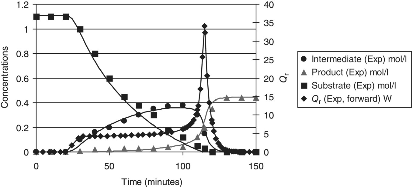
FIGURE 10.8 Concentration and heat flow profiles for Example Problem 10.3: symbols are measured data and curves are model predictions. A large spike in heat flow occurred at the end of the forward addition.
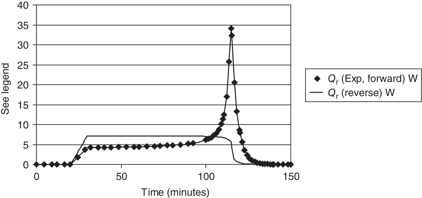
FIGURE 10.9 Heat flow profiles for Example Problem 10.3, comparing forward and reverse addition: symbols are measured data (forward addition) and curves are model predictions (forward and reverse addition). The heat flow curve indicates dosing‐controlled conditions when the addition is reversed.
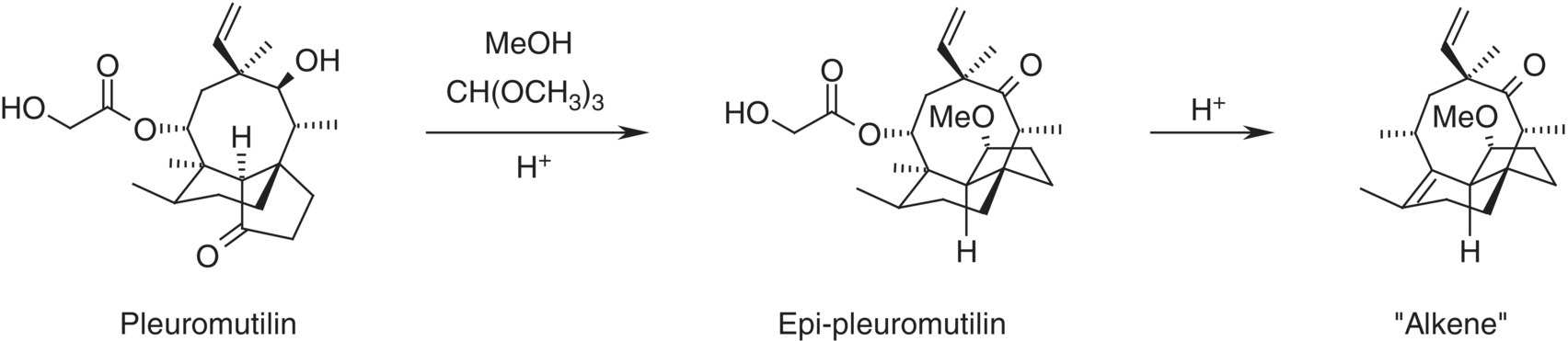
FIGURE 10.10 Overall reaction scheme for Example Problem 10.4 (epi‐pleuromutilin).
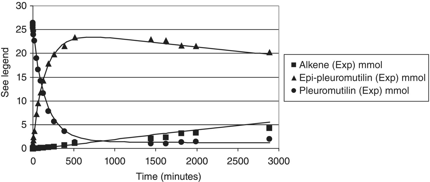
FIGURE 10.11 Typical reaction profiles for Example Problem 10.4. Symbols are measured data (from HPLC area percent) and curves are model predictions.
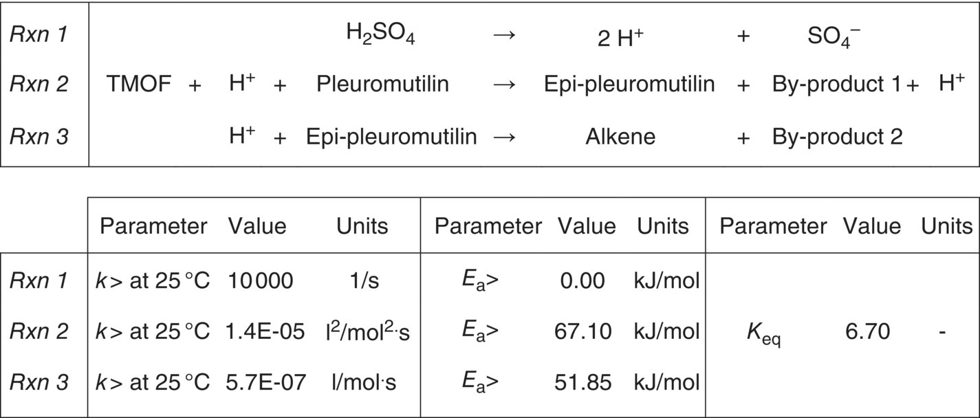
FIGURE 10.12 Final reaction scheme, rate constants, and activation energies for Example Problem 10.4 (epi‐pleuromutilin).
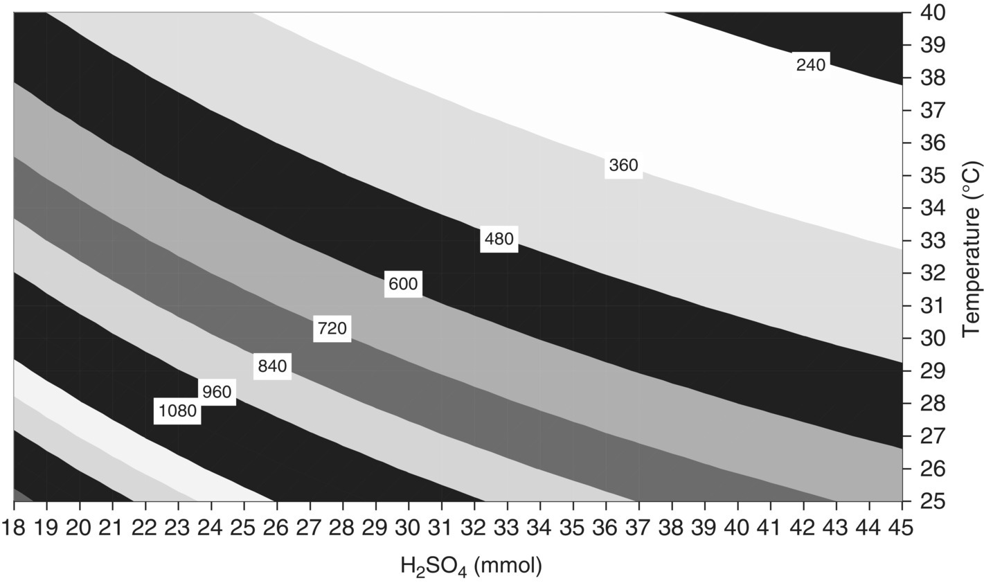
FIGURE 10.13 Response surface of ProductMaxTime (minutes) versus initial amount of acid and temperature (1 equiv. = 26.5 mmol) for Example Problem 10.4. Results produced using mechanistic model to run 440 virtual experiments.
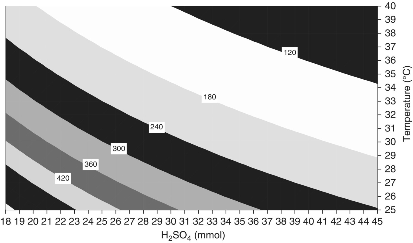
FIGURE 10.14 Response surface of QuenchWindow (minutes) versus initial amount of acid and temperature (1 equiv. = 26.5 mmol) for Example Problem 10.4. Results produced using mechanistic model to run 440 virtual experiments.
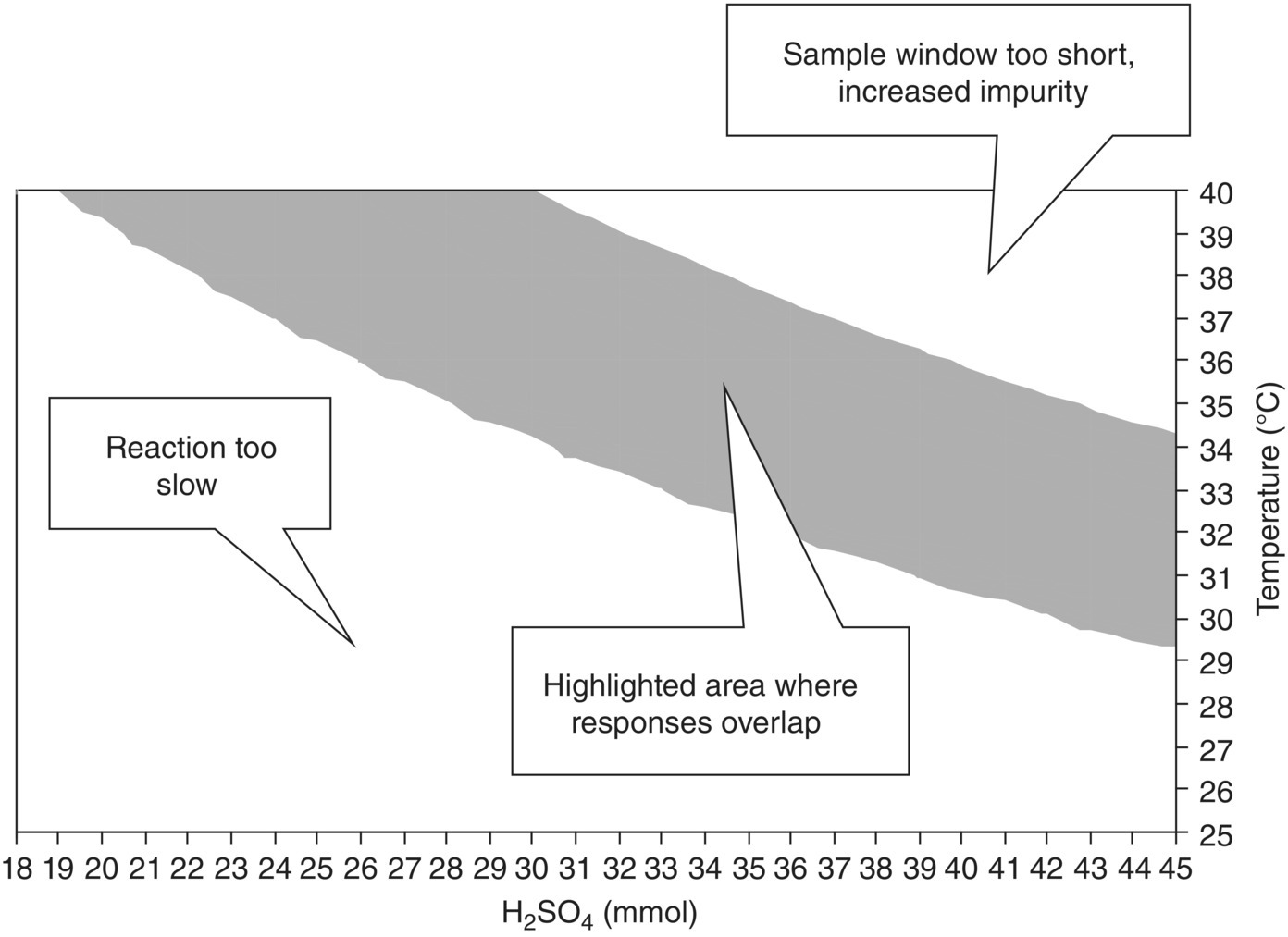
FIGURE 10.15 Region of overlapping response surfaces when ProductMaxTime and QuenchWindow are within specification, versus initial amount of acid and temperature (1 equiv. = 26.5 mmol) for Example Problem 10.4.
The original publication in 2007 [18] was based on 30 virtual simulations to which a polynomial equation was fitted for plotting; the above figures were reproduced in 2009 by running 440 virtual experiments in the same factor space with no interpolation.
Because kinetics limit this reaction at or near current operating conditions and because most of the reaction occurs after the addition, a scale‐independent design space for these responses may be constructed using two variables: temperature and equivalents of acid. When all other input material quantities are held constant and adequate temperature control is maintained on scale, the result of this reaction at any point in this space would be independent of scale.
Figure 10.15 is quite typical in that there appear to be two “edges of failure” when the responses are overlapped [27]. One response relates to the quality attribute (amount of alkene in this case), and another relates in this case to a business attribute (reaction time). In a strictly QbD context, Figure 10.15 therefore has only one edge of failure: if the quench window is too short, the alkene level will exceed its limit; if the reaction time is too long, this will not directly impact quality but will slow productivity.
The design space shown in Figure 10.15 is approximately 10 mmol wide and 5° high. However if a rectangular region of proven acceptable ranges had to be defined inside this space, the maximum width would be 7 mmol, and the maximum height 2–3°. This illustrates how the design space has the potential to offer greater flexibility than rigidly defined proven acceptable ranges.
On the other hand, Figure 10.15 remains quite restrictive, in that all other factors (such as substrate concentration) have to be held constant for it to apply. This is one of the reasons why a more dynamic design space definition based on the full mechanistic model, rather than one set of response surfaces at otherwise fixed conditions, has been advocated by industry [13]. The model verification statistics associated with this example are discussed at the end of this chapter.
10.5 APPLICATION TO CONTINUOUS FLOW SYSTEMS
Continuous flow reactor systems are of interest in API synthesis for the potential benefits they offer in certain cases relative to batch or fed‐batch reactors. These benefits may include greater process safety due to reduced holdup of hazardous material and the ability to quench a reaction more rapidly, improved containment of materials with low exposure limits, and reductions in capital and/or operating costs and volumetric productivity. In general, knowledge of the rate of reaction is even more important for design of continuous systems than for batch, as the residence time of the reactor is finite and it may be difficult to stop reaction sufficiently rapidly if problems arise. The economics of low volume production in a dedicated unit may limit the scope for continuous operation. Process issues specific to each application may also present challenges when reactors are operated for longer than typical batch cycle times, such as catalyst deactivation and difficulties handling slurries.
10.5.1 Plug Flow
Equations presented above for batch reactions may be applied directly to plug flow reactions after noting that the independent time variable now applies to position along the reactor [28]:
Here V is the cumulative volume of the reactor since the material entered at time zero and Q is the volume flow rate. When a plug flow reactor is operated at the same temperature and with the same residence time as a batch reactor with that cycle time, the end results are the same. This convenient result means that data collected in batch mode may be used for design in continuous mode and vice versa.
Plug flow reactors may be used for homogeneous systems, liquid–liquid and gas–liquid systems, with appropriate attention to ensuring that the phases are dispersed and separated when required and that both phases travel along the tube without accumulation.
Reaction characterization experiments follow the same logic as the corresponding problems in batch systems described above [14]. Equipment performance characterization in terms of heat transfer is always required; mixing and mass transfer characterization will be required when kinetics are rapid and in multiphase systems [14, 29]. Design spaces are expressed by taking into account similar factors to batch reactors.
Plug flow reactors with multiple addition points along the reactor length are analogous to fed‐batch systems with multiple sequential additions and likewise may be characterized and predicted using a similar approach to fed‐batch systems.
Useful additional information on application of continuous flow systems for API is available in the Refs. [30–32].
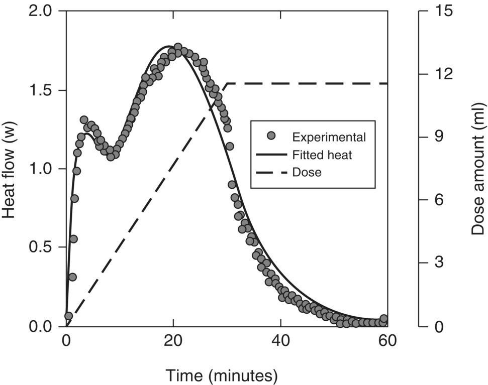
FIGURE 10.16 Fed batch heat flow data (discrete points) for peroxide oxidation reaction in Example Problem 10.5, showing double peak in heat output. Kinetic model results (curves) were used to design an intrinsically safer continuous reactor system.
10.5.2 CSTRs in Series
Plug flow behavior may be approximated using a cascade of stirred reactors in series [21]; this can also ease the problem of running slurry reactions in continuous mode. The approach to reaction characterization and design for these systems is described above. Equipment characterization in terms of heat transfer is always required, and batch characterization tests may be used for this purpose (see below).
Models developed for process prediction in batch or fed‐batch systems may be reused to design continuous stirred tank reactor systems by adding appropriate feeding and removal between reactors in the cascade [34]. When the number of reactors is large, a simpler plug flow model will give almost equivalent results.
10.6 EQUIPMENT CHARACTERIZATION AND ASSESSMENT
Equipment performance characteristics play a major role in most operations in API synthesis including each of the reaction types described above. This section reviews methods to evaluate some of the key characteristics for reactions, quenches, extractions, distillation/solvent swap, and crystallization.
Equipment performance can in general be quantified using either or both of the following methods:
- Characterization tests, in which purpose‐designed tests are carried out on the equipment and responses such as pressure, temperature, or concentration, are monitored versus time.
- Assessment calculations, in which empirical correlations, often based on dimensionless groups, are used to estimate equipment performance as a function of dimensions, geometry, fluid properties, and the intended operating volume and recipe.
Pharma API development laboratories, kilo labs, pilot plants, and full‐scale manufacturing plants are dominated by relatively standard, multipurpose equipment into which each new process is fitted; this means that performance data can be reused many times over once generated. To support QbD, equipment performance characteristics are stored in equipment databases that allow users at any location to retrieve performance data for equipment at both their own and other locations.
10.6.1 Heat Transfer
The product of overall heat transfer coefficient U and wetted area A appears throughout this chapter as equipment characteristics required for process scale‐up.
The product UA is best evaluated using a solvent test in the intended process vessel, to which solvent is charged and the fill level and agitator speed are set to those of the intended process. The batch is heated and/or cooled over the range of pot and jacket temperatures required by the process. Pot and jacket inlet temperatures are monitored continuously; jacket outlet temperature is monitored if available. In the absence of reaction and any other heat effects, Eq. (10.5) may be used to fit UA for both heating and cooling.
UA may also be estimated from chemical engineering correlations developed from measurements in similar types of equipment [35]. The coefficients in such heat transfer correlations may vary depending on the precise configuration, and in some cases, new coefficients may be required to describe unusual vessel configurations. In mature applications of equipment characterization, those coefficients are stored with the equipment configuration data in an equipment database for future reuse.
10.6.2 Mass Transfer
The product of mass transfer coefficient kL and interfacial area a (per unit volume) appears in this chapter whenever interphase transfer is involved.
The product kLa is best evaluated using a test in the intended process vessel, in which mass transfer either is the only phenomenon occurring or is the rate‐limiting phenomenon.
In one such test for headspace fed gas–liquid reactions, typically hydrogenations [36], solvent is charged, and the fill level set to that of the intended process. The headspace is evacuated and then pressurized with gas, and the agitator is turned on, with the speed increasing quickly to the intended process speed. Headspace pressure and both headspace and liquid temperature are monitored continuously. In the absence of reaction and any other phase transfer effects, Eq. (10.17) may be used to fit both gas–liquid (surface gassing) kLa and solubility. Alternatively, a reaction that consumes the dissolving gas may be run under conditions of high catalyst loading, such that mass transfer is rate limiting; in this case, Eq. (10.9) may be used to fit kLa to an indicator of reaction progress, such as hydrogen uptake. Note that (i) the kLa for surface gassing is very sensitive to the submergence of the top impeller [37] and (ii) sparging gas may be of little value in a “dead‐end” system (i.e. unless gas is continuously removed from the headspace) and mass transfer due to surface gassing is more important.
The depressurization test described above must be done carefully in order to provide useful data; for example, the headspace and liquid must be at the same temperatures before the agitator is turned on, to avoid a pressure recovery due to heating of the gas by the liquid.
For solid–liquid and liquid–liquid reactions, analogous characterization tests in which the uptake of solute is monitored (e.g. by sampling the liquid) may be used, or a known fast chemical reaction may be run under conditions in which dissolution of solute is rate limiting. Equation (10.9) again provides the basis for fitting kLa to the monitored profiles.
Alternatively, empirical estimates may be made using chemical engineering correlations; for these, the molecular diffusion coefficient of the solute in the solvent is required, which limits applicability. A feature that makes solid–liquid systems somewhat easier to predict is that the wetted area does not change with stirrer speed once the solids are suspended, that is, unless the particles are broken as a result of agitation. For liquid–liquid systems, the effect of minor components on the droplet size and the resulting surface area can be very significant, making accurate estimates difficult.
In all operations involving contact between multiple phases, a certain minimum level of agitation is required (even if kinetics are slow) in order to ensure that a dispersion of one phase exists in the other. In sold–liquid and liquid–liquid systems, the minimum stirrer speeds at which such a dispersion is created may be estimated with greater certainty than kLa.
For solid–liquid systems, this level of agitation (NJS – the agitator speed that just suspends the solid particles) exposes the full surface area, and kLa on scale may be taken as approximately equivalent to that which applied in a lab experiment using the same raw materials at the same conditions in which all of the solids were suspended; therefore similar kLa can be achieved even if neither lab or plant kLa is known. NJS may be estimated for a variety of impeller and tank configurations [38].
For liquid–liquid systems, a balance must be struck between mass transfer rate (favored by small droplets) and subsequent quick phase separation (favored by large droplets). Operating at NJD – the agitator speed that just disperses the liquid droplets of one phase in the other – exposes significant surface area while reducing the likelihood of forming a stable emulsion; once again the kLa on scale may be taken as similar to that which applied in a lab experiment with the same raw material at the same conditions in which the liquids were just dispersed; therefore similar kLa can be achieved even if neither lab or plant kLa is known. NJD may be estimated for a variety of impeller and tank configurations [34, 39].
If solid–liquid or liquid kLa is a factor in definition of a design space, the proximity of agitator speed to NJS or NJD, respectively, is a reasonable surrogate variable for kLa; for example, a dimensionless agitator speed that is scale independent could be defined as a factor:
N* in Eq. (10.37) might, for example, in a particular application need to be above 1.0 in order to avoid mass transfer limitations.
10.6.3 Liquid Mixing
In batch homogeneous reactions there is the possibility of reaction rate limitation by macromixing, at very low agitation rates. A macromixing time constant 30–60 seconds should eliminate this dependence, and correlations are available to estimate this factor [40]. The liquid mixing characteristics relevant for fed‐batch reactions are meso‐ and micromixing time constants; these appear in equations that describe the rate of localized mixing near the addition point in fed‐batch and continuous reactors and may be rate determining when kinetics are fast, i.e. for pseudo‐homogeneous, dosing‐controlled reactions as described above.
The time constants for meso‐ and micromixing may be characterized by running tests reactions with known kinetics in the target equipment [14, 41]. The outcome of these reactions is mixing sensitive under certain conditions and varies with factors such as impeller speed, addition rate, and addition location. When the product distribution or selectivity from each experiment is combined with a mathematical model based on Figure 10.7, the time constants for meso‐ or micromixing for each set of conditions may be obtained.
Alternatively, formulas are available for these time constants [14], and if the spatial distribution of the local rate of energy dissipation, ε, is known, the time constants may be obtained from these. Specialized tools such as computational fluid dynamics or laser anemometry may be used to estimate the spatial distribution of ε. As a general rule, ε is a multiple (e.g. 10–100) of the vessel‐averaged power input per unit mass (W/kg) near the impeller and a fraction (e.g. 1–10%) of the average near the liquid surface.
In continuous plug flow reactor systems, the extent of “axial dispersion” or longitudinal mixing along the axis of the flow may be characterized using pulse or step response experiments. Given the small scale that often applies in continuous pharmaceutical production/flow chemistry, the flow regime is not always turbulent (e.g. small diameter tubes with concentrated materials flowing at low velocities). In general, long, thin tubes, whether coiled or straight, lead to a low level of axial dispersion, and inserts such as static mixers further enhance the degree of plug flow and reduce axial dispersion to the point where assuming idealized plug flow behavior is a good approximation. An extensive discussion on this topic is available [42] containing further detail of measurement techniques and results to support process development and scale‐up. Application of PFRs in “flow chemistry”/continuous manufacturing also allows operation at higher temperature and pressure than typical for batch reactors, and in this case, fluid properties may differ significantly from those at ambient conditions, resulting in typically lower residence times for a given mass flow rate, due to thermal expansion.
10.6.4 Phase Separation
Phase separation times, e.g. after a liquid–liquid reaction or extraction, are longer on scale that in the laboratory [43]. As a rough indicator, the separation time scales with the liquid depth, so a separation time of one minute in the laboratory can easily extend to one hour on scale. Excessive separation times can be avoided by avoiding the formation of very fine droplets or stable emulsions; operating a liquid–liquid reaction at or near NJD as described above represents a good balance between high mass transfer area and short phase separation time.
10.6.5 Gas Disengagement
When reactions evolve gas, the rate of gas evolution scales with the reaction volume, but the ability of the liquid surface to allow the gas to escape scales with the cross‐sectional area of the vessel. The maximum velocity of gas escape through the liquid surface is approximately 0.1 m/s [34], allowing the maximum volume flow rate of gas evolution to be estimated:
This can be converted into a molar rate using the ideal gas law
If the rate of reaction exceeds the maximum rate of gas evolution, significant foaming will occur, and in some cases material will be lost from the reaction vessel. This problem becomes more likely on scale, as the maximum rate of gas evolution per unit volume reduces:
Equation (10.40) indicates that the volumetric rate of reactions evolving gases may need to be reduced on scale (e.g. by slower feeding or otherwise) in order not to exceed the limitations imposed by the equipment.
For example, in a vessel of 2 L nominal volume with diameter 0.115 m, filled to a level of 1 L at 20 °C, the maximum volumetric rate of a reaction evolving 1 mol of gas (e.g. CO2) per mole of product without batch swelling is 0.1 × (1/0.104) × (1.013 25 × 105/8.314 × (273.15 + 20)) = 39.97 mol/m3·s ≈ 0.04 mol/l·s. The same process running in a 2000 L vessel with diameter 1.5 m at 1600 L batch size is limited to a rate of 0.1 × (1/1)(1.013 25 × 105/8.314 × (273.15 + 20)) = 4.16 mol/m3·s ≈ 0.004 mol/l·s, i.e. 10 times slower, to avoid batch swelling.
10.7 MODEL VERIFICATION STATISTICS
10.7.1 Parameter Uncertainty
All models or equations with parameters that are derived originally from experimental data have a degree of uncertainty associated with their calculations or predictions. This is true for calibration curves, regression lines, response surfaces generated by design of experiments, chemical engineering correlations for estimating equipment performance, models based on ordinary differential equations (such as many of the examples shown above), and those using partial differential equations (such as computational fluid dynamics, in which turbulence models, “wall laws,” and other model parameters are ultimately based on experimental data). Unless these latter models involving differential equations are integrated over a sufficiently fine “grid,” their uncertainty is further increased by lack of precision.
Once accepted as useful, models are often used without taking this uncertainty into account, but experienced practitioners will always allow a factor of safety to compensate for a margin of error, even if the size of that error is not known. When the original data and the model are both available, it is possible to use statistical methods to quantify the uncertainty level. This makes the potential deficiencies of the model more evident and explicit and may also focus further experimentation on reducing those uncertainties.
More details about how to calculate uncertainty are given elsewhere [44], and Figure 10.17 illustrates the typical situation for a linear model in which the slope and intercept have been fitted.
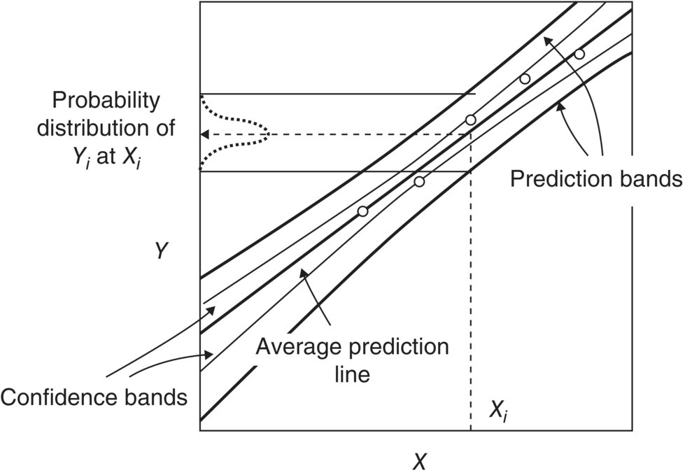
FIGURE 10.17 Schematic of confidence and prediction bands for a linear model in which the slope and intercept of the best fit line have been fitted to data (symbols).
Confidence bands define an envelope within which there is a certain confidence level (typically 95%) of the true location of the best‐fit line. Prediction bands (or intervals) define a wider envelope within which there is a certain confidence level (e.g. 95%) that all datapoints/observations will lie. The width of prediction bands relative to the model prediction indicates the likely relative error of the model predictions; this also reflects underlying variability or lack of reproducibility in the experimental data. For typical linear models such as that in Figure 10.17, the band widths are at a minimum at the center of the experimental data and increase in either direction from the center. This tallies with the belief that models are most applicable near the conditions where the experiments were run and become less reliable at more extreme conditions.
Any such model should in the first instance be based on reliable, reproducible data; there should also be sufficient data to avoid “overfitting,” i.e. the number of observations should be significantly greater than the number of model parameters fitted. The degree to which such a model can be said to be verified depends on the width of its prediction bands compared with the accuracy needed in the intended application.
For example, if a model predicts an impurity level of 0.1%, with 95% prediction band widths of 0.05%, one could state with a high degree of confidence that the impurity level will be less than 1%; more formally, the probability of impurity exceeding 1% is almost zero, p(Impurity > 1%) ≈ 0. The same model is not sufficiently accurate to state with the same degree of confidence that the impurity level will be less than 0.2%, i.e. p(Impurity > 0.2%) > 0. However if the 95% prediction band width was 0.01%, the model would be suitable for more confident predictions at lower impurity levels. There is therefore an element of fitness for purpose when judging whether a model has been verified sufficiently to apply it in a given situation.
Similarly, if the correlation used to calculate the stirrer speed required to suspend solids has a stated accuracy of 20% and the predicted NJS = 80 rpm, this level of verification is sufficient to say that 40 rpm is too little – p(Suspended) ≈ 0‐ and 120 rpm is too much – p(Suspended) ≈ 1, but not whether 75 rpm is sufficient – 0 < p(Suspended) < 1.
Returning to Example Problem 10.4, confidence and prediction bands may be calculated for a dynamic model based on chemical engineering rate equations, and typical results are shown in Figures 10.18 and 10.19.

FIGURE 10.18 Model predictions with confidence and prediction bands/limits for the product profile in Example Problem 10.4, compared with experimental measurements of that profile. All measured data lie within the envelope defined by the 95% prediction bands.
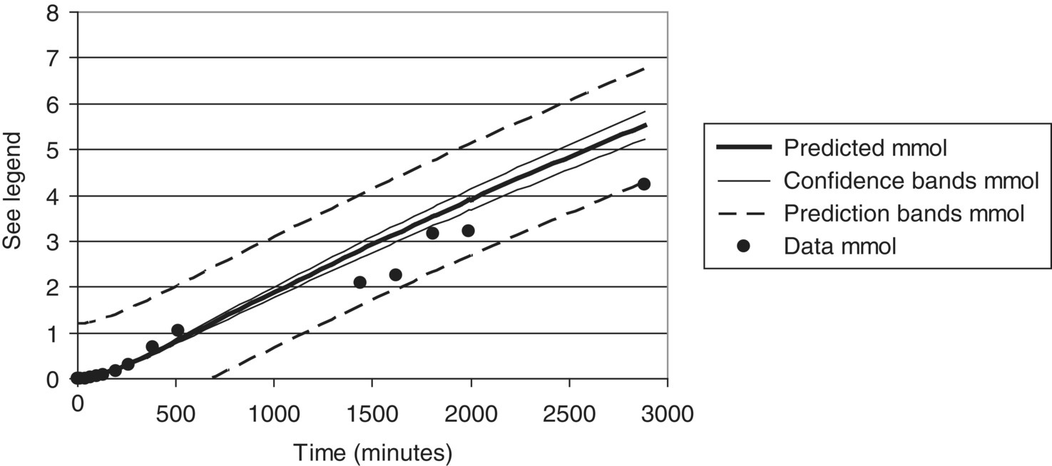
FIGURE 10.19 Model predictions with confidence and prediction bands/limits for the alkene profile in Example Problem 10.4, compared with experimental measurements of that profile. All measured data lie within the envelope defined by the 95% prediction bands.
Comparing Figures 10.18 and 10.19, the relative width of prediction bands is greater for alkene than for product. This reflects greater uncertainty in the alkene measurements and predictions.
In QbD work, the criticality of factors is sometimes judged according to their proximity to factor settings that define the “edge of failure,” e.g. crossing an impurity limit. Prediction bands should be taken into account when judging criticality in this way, as these will show that failure will occasionally occur at factor settings that are nearer to intended operating conditions.
10.7.2 Implications for Design Space Definition
The existence of uncertainty means that formal probability statements may be required to properly define a design space; while this implies some additional work, it has the benefit of quantifying the degree of assurance (or risk) that exists in relation to how the process will perform. In general, this approach will lead to design spaces that are smaller and more conservative than when uncertainty is ignored and that maximize the probability that the product quality will be in specification. Most popular statistical software packages at present do not take uncertainty into account in this way [45].
The relevant probability can be calculated in a variety of ways, and Figure 10.20 illustrates application to Example Problem 10.4. Recall from Figure 10.19 that the relative uncertainty of alkene is greater than that for product in this case; this leads to a relatively broader region of conditions in which the impurity has a significant probability of failing to meet specification. On the other hand, uncertainty in product predictions is low, leading to a narrow region separating success and failure. To produce Figure 10.20, the relative uncertainty in quench window was taken to be proportional to that of alkene and the relative uncertainty of ProductMaxTime proportional to that of product.
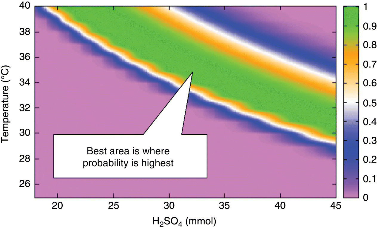
FIGURE 10.20 Response surface showing joint probability that responses ProductMaxTime and QuenchWindow will be in specification for Example Problem 10.4.
Figure 10.20 illustrates the regions of the factor space with the highest probability of success; these are the most favorable regions in which to operate the process. In the green area of Figure 10.20, the probability of success exceeds 80%. Figure 10.21 compares the design space defined on this basis (p > 80%) with that obtained by overlapping the average responses; as expected, taking account of uncertainty reduces the size of the design space.
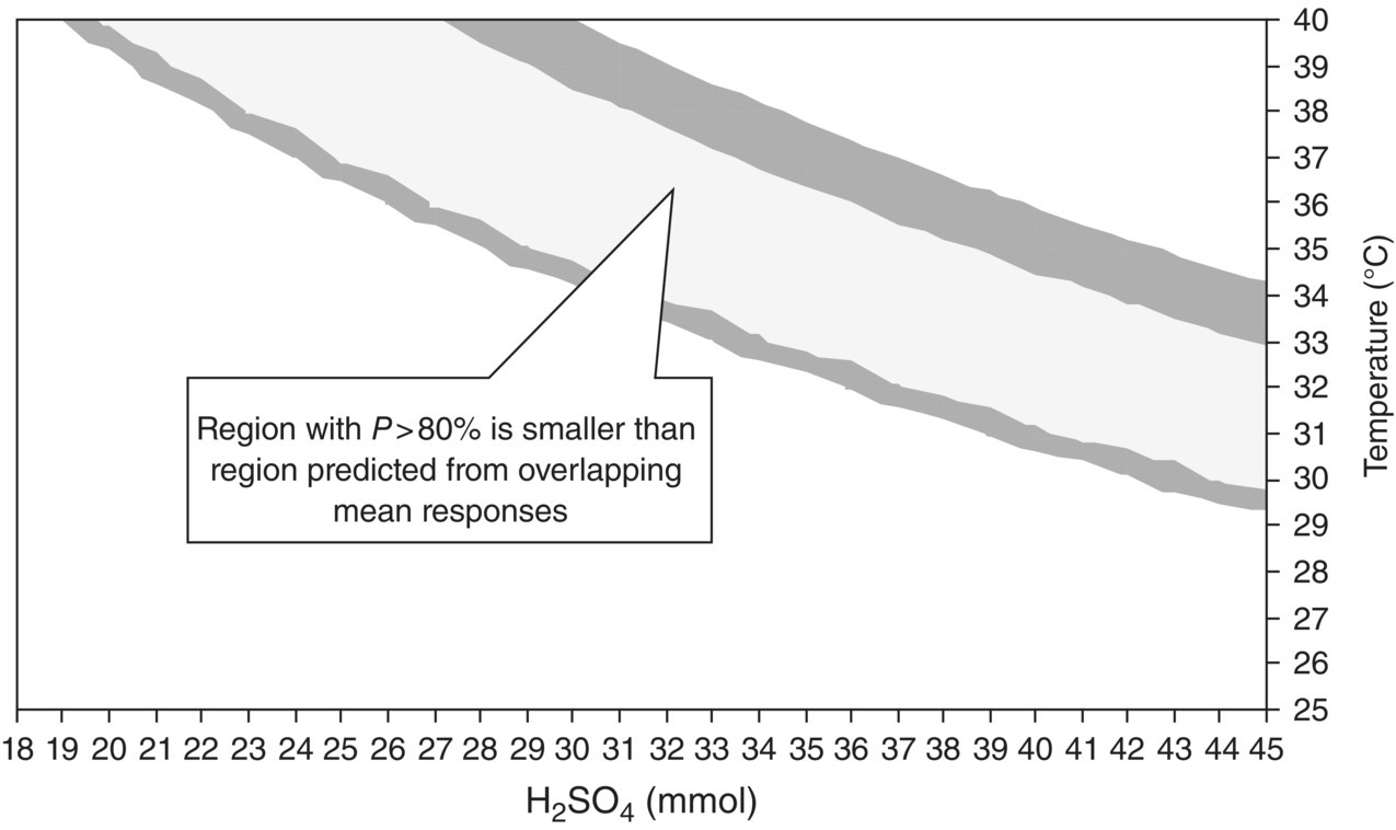
FIGURE 10.21 Comparison of design space for Example Problem 10.4 defined using average responses and that defined using probability of success greater than 80%.
The above results show that for QbD purposes, uncertainty in data or responses predicted by any model should be explicitly taken into account in defining the design space; probability is the natural way to do this. Uncertainty will tend to shrink the design space away from the edges of the area where average responses overlap, in line with good engineering practice. When the peak probability is far from 100%, this highlights the need to obtain greater process understanding, or an improved process, before proceeding.
10.8 NOTATIONS
| Symbol | Meaning | Units |
| a | Area per unit liquid volume | m2/m3 |
| α | Reaction order; also volume ratio | — |
| A | Area for heat transfer | m2 |
| β | Reaction order | — |
| C | Concentration; also specific heat capacity | mol/m3 (concentration) J/kg K (heat capacity) |
| D | Diameter | m |
| ΔT | Temperature difference | °C or K |
| ΔH | Heat of reaction | J/mol |
| E | Energy | J/mol |
| H | Henry’s law constant; also liquid depth | (Henry constant) m (liquid depth) |
| k | Rate constant; also mass transfer coefficient | m3/mol·s (kinetics) m/s (mass transfer) |
| N | Impeller rotational speed; also hydrogen supply rate | 1/s and rpm (impeller speed) mol/s (hydrogen supply rate) |
| ν | Stoichiometric coefficient | — |
| p | Pressure; also probability | Pa (pressure) ‐(probability) |
| Q | Volumetric flow rate; also heat flow rate | m3/s (flow rate) W (heat flow rate) |
| r | Rate of reaction | mol/m3s |
| ρ | Density | kg/m3 |
| R | Gas constant | J/mol·K |
| S | Partition coefficient | — |
| U | Overall heat transfer coefficient | W/m2K |
| V | Liquid volume | m3 |
| t | Time | s |
| T | Temperature; also tank diameter | K or °C (temperature) m (tank diameter) |
| Subscripts | ||
| 0 | Initial; also at infinite temperature | |
| A | Of component A; also of activation | |
| B | Of component B | |
| bulk | Of the bulk solution | |
| d | Of the dispersed phase | |
| H2 | Of hydrogen | |
| f | Of the feed | |
| fed | Of limiting fed reactant | |
| gas | Of gas | |
| head | Of the headspace | |
| i | Of the ith component | |
| ij | Of the ith component in the jth reaction | |
| j | At the inlet to the cooling jacket or coil; also of the jth reaction | |
| JS | Just suspended | |
| JD | Just dispersed | |
| L | In the liquid phase | |
| LM | Logarithmic mean | |
| m | Of mixing | |
| max | Maximum | |
| p | At constant pressure | |
| r | Of reaction | |
| solute | Of limiting dissolving solute | |
| transfer | Of reaction | |
| Superscripts | ||
| * | At saturation, i.e. equilibrium between the phases; also dimensionless | |
REFERENCES
- 1. ICH. (2012). International Conference on Harmonization (ICH) Q8, Q9, Q10 guidance documents. https://www.ich.org/products/guidelines/quality/article/quality‐guidelines.html (accessed 24 October 2018).
- 2. Place, D. (2009). Using DynoChem to determine a suitable sampling endpoint for reaction analysis in a DoE. DynoChem User Meeting, Philadelphia (14–15 May 2009). https://dcresources.scale‐up.com/?t=pu&id=223 (accessed 24 October 2018).
- 3. Hoffmann, W. (2015). Obtain reaction scheme proposal from chemical structures and HPLC data, training exercise published 1. https://dcresources.scale‐up.com/?t=tr&id=5306&pid=17 (accessed 24 October 2018).
- 4. Weires, N.A., Caspi, D.D., and Garg, N.K. (2017). Kinetic modeling of the nickel‐catalyzed esterification of amides. ACS Catal. 7 (7): 4381–4385.
- 5. Niemeier, J.K., Rothhaar, R.R., Vicenzi, J.T., and Werner, J.A. (2014). Application of kinetic modeling and competitive solvent hydrolysis in the development of a highly selective hydrolysis of a nitrile to an amide. Org. Process Res. Dev. 18 (3): 410–416.
- 6. Shujauddin, M. (2016). Changi and Sze‐Wing Wong, kinetics model for designing Grignard reactions in batch or flow operations. Org. Process Res. Dev. 20 (2): 525–539.
- 7. Mandrelli, F., Buco, A., Piccioni, L. et al. (2017). The scale‐up of continuous biphasic liquid/liquid reactions under super‐heating conditions: methodology and reactor design. Green Chem. 19: 1425–1430.
- 8. Ramirez, A., Hallow, D.M., Fenster, M.D.B. et al. (2016). Development of a control strategy for a final intermediate to enable impurities control. Org. Process Res. Dev. 20 (10): 1781–1791.
- 9. Vickery, T. (2007). Scale‐up from RC1 and ARC safety tests using DynoChem. DynoChem User Meeting, Philadelphia (15–16 May 2007). https://dcresources.scale‐up.com/?t=pu&id=264 (accessed 24 October 2018).
- 10. Bright, R., Dale, D.J., Dunn, P.J. et al. (2004). Identification of new catalysts to promote imidazolide couplings and optimisation of reaction conditions using kinetic modelling. Org. Proc. Res. Dev. 8 (6): 1054–1058.
- 11. Jorgensen, M. (2009). Modeling is the Easy Part!: getting the right data and getting the data right is the challenging part!. DynoChem User Meeting, Philadelphia (14–15 May 2009). https://dcresources.scale‐up.com/?t=pu&id=212 (accessed 24 October 2018).
- 12. Eyley, S. (2009). Why study a synthetically useless reaction? Unravelling sulphonate ester formation using DynoChem. DynoChem User Meeting, Philadelphia (14–15 May 2009). https://dcresources.scale‐up.com/?t=pu&id=212 (accessed 24 October 2018).
- 13. Niemeier, J. (2009). Using DynoChem to scale up data from various calorimeters. DynoChem User Meeting, Philadelphia (14–15 May 2009). https://dcresources.scale‐up.com/?t=pu&id=217 (accessed 24 October 2018).
- 14. Nyrop, J. (2009). Development of a high performance, company specific DynoChem front‐end. DynoChem User Meeting, Philadelphia (14–15 May 2009). https://dcresources.scale‐up.com/?t=pu&id=218 (accessed 24 October 2018).
- 15. Hannon, J., Hearn, S., and Brechtelsbauer, C. (2002). Characterisation of the scalability of hydrogenation reactions. Scientific Update Scale‐up Conference, St Helier, Jersey (23–26 September 2002). https://dcresources.scale‐up.com/?t=pu&id=281 (accessed 24 October 2018).
- 16. Remy, B., Brueggemeier, S., Marchut, A. et al. (2008). Modeling‐based approach towards on‐scale implementation of a methanethiol‐emitting reaction. Org. Process Res. Dev. 12: 381–391.
- 17. Richter, S. and Allian, A. (2008). Process safety testing and process modeling in the PSL using DynoChem. 3rd US Pharmaceutical Process Safety Forum, Pearl River, New York (14 October 2008). https://dcresources.scale‐up.com/?t=pu&id=235 (accessed 24 October 2018).
- 18. Hannon, J. (2008). Design space for a synthesis reaction, Part 3. http://blog.scale‐up.com/2008/04/design‐space‐for‐synthesis‐reaction.html (accessed 24 October 2018).
- 19. Stonestreet, P., Hodnett, N., Squires, B., and Escott, R. (2009). Roles of mechanistic and empirical modeling/DOE in achieving Quality by Design. DynoChem User Meeting, Philadelphia (14–15 May 2009). https://dcresources.scale‐up.com/?t=pu&id=216 (accessed 24 October 2018).
- 20. Baldyga, J., Bourne, J.R., and Hearn, S.J. (1997). Interaction between chemical reactions and mixing on various scales. Chem. Eng. Sci. 52 (4): 457–466.
- 21. Hoffmann, W. (2007). DynoChem and homogeneous mixing: an example. DynoChem user Meeting, Philadelphia (15–16 May 2007). https://dcresources.scale‐up.com/?t=pu&id=266 (accessed 24 October 2018).
- 22. Hoffmann, W. (2001). Workshop on Basics of Kinetics/Application of Software Tools, Introduction to the determination of kinetic parameters. Mettler Toledo RXE Forum, Lucerne 2001.
- 23. Hallow, D., Mudryk, B., Braem, A. et al. (2009). Application of DynoChem® reaction modeling to quality by design. DynoChem User Meeting, Philadelphia (15–21 November 2008). https://aiche.confex.com/aiche/2008/techprogram/P135622.htm (accessed 24 October 2018).
- 24. Wertman, J. (2007). GSK approach to enhancing process understanding using DynoChem: reaction kinetics examples. DynoChem User Meeting, Philadelphia (15–16 May 2007). https://dcresources.scale‐up.com/?t=pu&id=258 (accessed 24 October 2018).
- 25. Hannon, J. (2009). Quality by design for drug substance scale‐up. Presented at Scientific Update Conference on Scale‐up of Chemical Processes, Vancouver, Canada (7–10 July 2009). https://dcresources.scale‐up.com/?t=pu&id=205 (accessed 24 October 2018).
- 26. Akaike, H. (1974). A new look at the statistical model identification. IEEE Trans. Autom. Control 19 (6): 716–723.
- 27. am Ende, D., Bronk, K.S., Mustakis, J. et al. (2007). API quality by design example from the torcetrapib manufacturing process. J. Pharm. Innov. 2: 71–86.
- 28. Levenspiel, O. (1999). Chemical Reaction Engineering, 3e. New York: Wiley.
- 29. Zhu, Z.M., Hannon, J., and Green, A. (1992). Use of high intensity gas‐liquid mixers as reactors. Chem. Eng. Sci. 47: 2847–2852.
- 30. am Ende, D. (2009). Lean and green, the value of API process design. DynoChem User Meeting, Philadelphia (14–15 May 2009). https://dcresources.scale‐up.com/?t=pu&id=220 (accessed 24 October 2018).
- 31. Roberge, D., Gottsponer, M., Eyholzer, M., and Kockmann, N. (2009). Industrial design, scale‐up, and use of microreactors. Chemistry Today 27 (4): 8–11.
- 32. Ford, D. (2015). Using data‐rich experimentation to enable the development of continuous processes. Mettler Toledo Symposium, Cambridge (20 May 2015). https://dcresources.scale‐up.com/?t=pu&id=6063 (accessed 24 October 2018).
- 33. Chan, S.H., Wang, S.S.Y., and Kiang, S. (2005). Modeling and alternative reactor design for a highly exothermic reactive system. AIChE Annual Meeting, Cincinnati, OH (30 October to 4 November 2005).
- 34. Erdman, D. (2009). DynoChem modelling of 3 continuous stirred tank reactors. DynoChem User Meeting, Philadelphia (14–15 May 2009). https://dcresources.scale‐up.com/?t=pu&id=221 (accessed 24 October 2018).
- 35. Kayode Coker, A. (2001). Modeling of Chemical Kinetics and Reactor Design. Houston, TX: Gulf Professional Publishing.
- 36. Machado, R. (1994). Fundamentals of mass transfer and kinetics for the hydrogenation of nitrobenzene to aniline. Presented at 7th RC User Forum USA, St Petersburg Beach (23–26 October 1994).
- 37. Lines, P.C. (2000). Gas‐liquid mass transfer using surface‐aeration in stirred vessels, with dual impellers. Chem. Eng. Res. Des. 78: 342–347.
- 38. Zwietering, T.N. (1958). Suspending of solid particles in liquid by agitators. Chem. Eng. Sci. 8: 244.
- 39. Lines, P.C. and Carpenter, K.J. (1990). The effect of physical property ranges on correlations for minimum impeller speeds to disperse immiscible liquid mixtures. IChemE Symp. Series 121: 167–182.
- 40. Paul, E.L., Atiemo‐Obeng, V.A., and Kresta, S.M. (2004). Handbook of Industrial Mixing. Hoboken, NJ: Wiley.
- 41. Bourne, J.R. and Yu, S. (1994). Investigation of micromixing in stirred tank reactors using parallel reactions. Ind. Eng. Chem. Res. 33 (1): 41–55.
- 42. May, S.A., Johnson, M.D., Braden, T.M. et al. (2012). Rapid development and scale‐up of a 1H‐4‐substituted imidazole intermediate enabled by chemistry in continuous plug flow reactors. Org. Process Res. Dev. 16: 982–1002.
- 43. Atherton, J.H. and Carpenter, K. (1999). Process Development: Physiochemical Concepts. Oxford: Oxford Science.
- 44. Box, G.E.P., Hunter, W.G., and Stuart Hunter, J. (1978). Statistics for Experimenters: An Introduction to Design, Data Analysis, and Model Building. Hoboken, NJ: Wiley.
- 45. Peterson, J.J. (2008). A Bayesian approach to the ICH Q8 definition of design space. J. Biopharm. Stat. 18 (5): 959–975.