50
DEVELOPMENT OF DESIGN SPACE FOR REACTION STEPS: APPROACHES AND CASE STUDIES FOR IMPURITY CONTROL
Srinivas Tummala, Antonio Ramirez, and Sushil Srivastava
Bristol‐Myers Squibb, New Brunswick, NJ, USA
Daniel M. Hallow
Noramco, Athens, GA, USA
50.1 INTRODUCTION
The objective of pharmaceutical development is to advance a commercial manufacturing process to consistently deliver drug substance and drug product of the intended quality through the life cycle of the product [1]. The scientific knowledge gained from pharmaceutical development and manufacturing experience provides understanding to enable process optimization and support the establishment of chemistry and manufacturing controls that assure product quality. Elements of the control strategy can include drug substance specifications, procedural controls, controls in material attributes (MAs), and parameter controls. In the case of parameter controls, the selection of ranges that provide material meeting quality criteria can be presented in terms of univariate intervals that keep other parameters at their intended target value. Alternatively, the parameter range selection can be built upon multivariate experimentation to define a design space, “the multidimensional combination and interaction of input variables and process parameters that has been demonstrated to provide assurance of quality”[2].
Although there is no regulatory requirement for the establishment of a design space to define a successful control strategy, design space selection is associated with an enhanced approach to pharmaceutical development that can provide a more robust process and lead to regulatory flexibility. For example, working within an approved design space is not considered an operational change and could facilitate continuous improvement throughout the product life cycle. A design space is proposed by the applicant as part of the regulatory submission and subject to the approval of the regulatory agencies.
This chapter examines current approaches to establish a design space for reaction steps. The review does not intend to give an exhaustive description but rather distill key concepts from existing ICH guidance and illustrate them with case studies. Certainly, the selection of these examples is biased by the author's interests and experience. Efforts to maintain a uniform terminology throughout the chapter were made for the sake of clarity but may have not captured subtle modifications due to varying approaches specific to different companies, processes, or products.
50.2 ELEMENTS OF PHARMACEUTICAL DEVELOPMENT
50.2.1 Quality Target Product Profile
The first step toward achieving the goals of pharmaceutical development is to outline a summary of the characteristics of the drug product that will ideally be achieved to ensure the desired quality from a safety and efficacy perspective. These characteristics are commonly referred to as the quality target product profile (QTPP). The mode of delivery, dosage strength, factors that impact release of the therapeutic moiety, and the drug product quality attributes (QAs) (e.g. sterility, purity, and stability) must be considered when assessing the QTPP. In order to guarantee product safety and efficacy for the patient, only characteristics pertinent to the patient should be included in the QTPP. For example, if particle size is critical to the dissolution of an oral solid product, the QTPP should refer to dissolution instead of particle size [3]. A typical example of QTPP for an oral solid dosage product is described in Table 50.1.
TABLE 50.1 Example of QTPP for an Oral Solid Dosage Product
| QTPP | Target | Justification |
| Dosage form | Capsule | Proven effective dosage form |
| Dosage design | Immediate release soft gelatin capsule | Efficacy of the drug product |
| Dosage strength | 100 mg | Efficacy of the drug product |
| Route of administration | Oral | Safe and effective route |
| Identity | Drug substance is “name” | Safety of the drug product |
| Assay | 95–105% | Efficacy of the drug product |
| Impurity profile | Control of potential impurities in drug substance | Safety of the drug product |
50.2.2 Potential Critical Quality Attributes
The potential critical quality attributes (pCQAs) of the drug product and, subsequently, those of the drug substance are identified based on the QTPP and initial process knowledge. ICH Q8 defines a CQA as “a physical, chemical, biological, or microbiological property or characteristic that should be within an appropriate limit, range, or distribution to ensure the desired product quality.” CQAs of an oral solid dosage product typically include characteristics affecting product purity, strength, drug release, and stability. For a drug substance, the pCQAs include those properties that could potentially affect drug product CQAs. The first column of Table 50.2 illustrates common pCQAs for a drug substance.
TABLE 50.2 Example of pCQAs for an Oral Solid Drug Substance
| Quality Attribute | Tests | Criticality | Rationale |
| Identity | IR/Raman/HPLC | Yes | ICH Q6A |
| Assay | HPLC | Yes | Impacts drug product potency |
| Impurity | |||
| Related substances | HPLC | Yes | Impurity x in the Final Intermediate has potential to impact drug substance quality and is controlled to ≤0.20 RAP |
| Genotoxic impurities | LC‐MS | Yes | Residual y and p‐TsOEt are GTIs. These impurities are controlled below the TTC limits, i.e. ≤3.7 ppm each for y and p‐TsOEt |
| Diastereomers | HPLC | Yes | ICH Q6A Flowchart #5 “z” is an optically active substance |
| Inorganic impurities (including heavy metals) | ICP‐MS | No | No metals used in the synthesis of the drug substance. The level of inorganic impurities is controlled at ≤20 ppm |
| Class 2 residual solvents | GC | Yes | Class 2 solvents are used in the manufacturing process. These solvents are controlled below limits defined in ICH Q3 (R6) |
| Particle size distribution | LLS | No | Drug substance is dissolved during drug product manufacture |
| Solid‐state crystal form | PXRD | No | Drug substance is dissolved during drug product manufacture |
The TTC acronym stands for “Threshold of Toxicological Concern” for genotoxic impurities. See Section 50.7.
Impurities are a fundamental class of drug substance pCQAs due to their ability to impact the safety and efficacy of the drug product. For chemical entities, impurities can involve organic impurities – including potentially genotoxic impurities (GTIs) [4], inorganic impurities (e.g. residual metals), and residual solvents. Understanding the key steps where the impurities form and purge in the process and establishing controls to ensure that these impurities do not affect the quality of the drug substance is a key focus of drug substance development.
50.2.3 Quality Risk Assessment
Quality risk assessment is a tool used to (i) evaluate if a pCQA is likely to impact quality, (ii) review which steps of the synthesis are likely to affect these CQAs, and (iii) identify and rank MAs and process parameters that may influence the QAs of the step's output and ultimately impact drug substance quality. The characteristics of an input material that should be within an appropriate limit, range, or distribution to ensure the desired product quality are commonly referred to as MAs [5]. For a discussion of quality risk assessment in drug substance process development, see Chapter 49.
A criticality assessment – a yes or no evaluation primarily based on severity of harm – is employed to determine which of the potential CQAs of the drug substance are likely to impact the drug product CQAs. This assessment does not change as a result of risk management [6] and is iterative in nature because criticality of the pCQAs may evolve during process development: as process knowledge increases, the evaluation of the impact of a pCQA on the quality of the drug product may change. The last two columns of Table 50.2 illustrate a criticality assessment and its rationale for pCQAs.
Once the synthesis for the commercial process is established, a collective process risk assessment is carried out to identify the steps in the synthetic sequence whose QAs have the potential to impact drug substance quality. These steps can be designated as “critical steps.” For most early steps, the assessment focuses on evaluating if impurities from these steps impact the drug substance impurity pCQAs. Typical levels of impurities in a given step are evaluated for their fate and purge in the subsequent unit operations. Criticality of a process‐related impurity can only be established when the functional relationship between the impurity and the drug substance pCQA is mapped and understood. For the final steps, additional properties are assessed beside impurity profile, including physical properties of the drug substance pCQAs such as crystal form, particle size, etc. Finally, an individual risk assessment of each step is performed to assess MAs and process parameters that could impact the QAs of that step. MAs and process parameters are then prioritized for additional investigation.
50.2.4 Control Strategy
A central tenet of the quality‐by‐design (QbD) paradigm for process development is to understand the relationship between MAs and process parameters and the QAs for the various steps in the synthesis. Subsequent sections of this chapter will outline two methodologies to establish this link, namely, the mechanistic approach and the empirical approach. If cause–effect analysis demonstrates that there is a link between the MAs, process parameters, or both and the QAs, then a control strategy must be developed to ensure that consistent quality can be achieved. The control strategy for the impurity CQA can entail one or several of the following elements: (i) specifications for the input materials; (ii) specifications for impurities in the starting materials and intermediates of the chemical synthesis based on fate and purge during the process; (iii) process design to mitigate impurity formation, purge of the impurity, or both; and (iv) ranges for MAs and process parameter controls to reduce impurity formation or ensure its purge in subsequent processing steps [7]. A representative flow diagram of elements of pharmaceutical development in drug substance manufacture is shown in Figure 50.1.

FIGURE 50.1 Elements of pharmaceutical development in drug substance manufacture. DP, drug product; DS, drug substance; QAs, quality attributes of a given step; PPs, process parameters; MAs, material attributes.
50.2.4.1 Proven Acceptable Ranges and Design Space
The ranges for MAs and process parameters in which quality is assured can be expressed either as a series of proven acceptable ranges (PARs) or as a multivariate design space. PARs for a given parameter denote the univariate range that the parameter could vary within and still assure quality either because (i) it has minimal or no interaction with other MAs and process parameters on how it impacts the quality attribute or (ii) it assumes that all the other attributes and parameters are at or close to their target values. When parameters have significant multivariate interactions, the ranges can be expressed as a design space. The final control strategy may include a mixture of PARs, design spaces, or both across the unit operations and reaction steps. Choosing the approach for each operation should consider the risk and impact of multivariate interactions on product quality. The normal operating range (NOR) of a parameter corresponds to the manufacturing range inside the PAR that is defined by the target value and extent in which the parameter is controlled (Figure 50.2) [8].
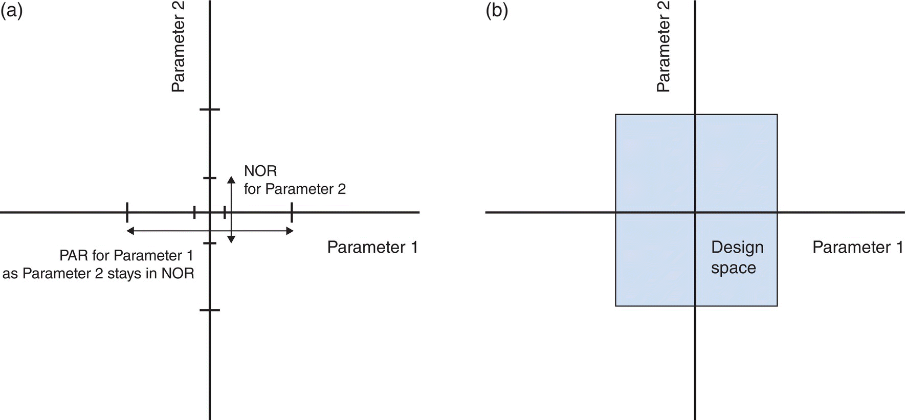
FIGURE 50.2 Depiction of (a) proven acceptable ranges and (b) a two‐dimensional design space.
50.2.4.2 Unit Operation Design Space
Impurities with potential impact on the quality of the drug substance can (i) originate from input raw materials, (ii) form in earlier steps of the synthesis, or (iii) be generated in the drug substance step. During the assessment of the impact of MAs and process parameters on the QAs of a step, dividing the step into unit operations helps to decide which operations should be selected for further evaluation. Let us consider an intermediate step that generates an impurity with potential to impact the QAs (Eqs. 50.1 and 50.2, Table 50.3). The reaction that forms the impurity and the crystallization that purges it can be chosen for additional analysis. Establishing limits for the impurity levels that must be met at the end of the reaction and after the crystallization facilitates the independent study of the operations – i.e. understanding the impact of the process parameters and defining process parameter ranges or design spaces that assure quality. The following sections of this chapter focus on reaction steps:
TABLE 50.3 Representative Assessment of Unit Operations
| Unit Operation | Assessment | Potential to Impact QAs |
| Reaction | Impurity formation step | High |
| Quench, extraction, washes | Minimal impact on Impurity level | Low |
| Distillation | Minimal impact on Impurity level | Low |
| Crystallization | Impacts Impurity purge level | Medium |
| Drying | Minimal impact on Impurity level | Low |
50.3 REACTION DESIGN SPACE DEVELOPMENT
50.3.1 Establishing Functional Relationships
While the development of the steps in the synthesis of a drug substance must consider all the unit operations, the reaction step assumes significance because it often is the origin of the impurities that could be quality impacting. As discussed previously, an individual risk assessment of the reaction step is carried out to identify the MAs and process parameters that can impact impurity levels. Subsequently, the functional relationship between these impurities, MAs, and process parameters needs to be established. This relation can be determined using a univariate analysis in which the effect of a single variable on a given quality attribute is measured while keeping the other variables at their “target” value. Alternatively, the relationship can be established using a multivariate analysis that considers the effect of multiple variables at a time.
Two strategies based on the elaboration of predictive models can be adopted to define a multivariate functional relationship: the mechanistic and the empirical approach. Mechanistic models entail the elucidation of kinetic and thermodynamic expressions that define the formation of product and relevant impurities. In contrast, empirical models utilize design of experiment (DOE) [9] and statistical analysis to regress polynomial expressions that help establish the desired relationship. From an ideal standpoint, the mechanistic approach would be the preferred strategy since it is underpinned by fundamental knowledge. However, in complex systems where developing a full understanding is not viable, the empirical approach may be employed [10].
50.3.2 Development of the Mechanistic Model
Mechanistic models for a reaction step correlate concentrations of the species involved in the transformation with the underlying processes and variables deemed to affect them, according to physical organic principles. The models aim at describing the time‐course fate of input materials, intermediates, and products and require an understanding of the elementary steps that represent the reaction, including kinetic and thermodynamic variables. The development of a mechanistic model involves four basic stages: (i) description of the elementary steps that define the transformations of interest, (ii) mechanistic studies to define model variables, (iii) regression of model variables using an experimental building data set, and (iv) model evaluation using an experimental verification data set.
50.3.2.1 Description of Elementary Steps
Model development starts by defining the sequence of elementary steps that represents the overall reaction. Literature precedence, control experiments, or a combination of both can be used to lay out the adequate network of discrete processes that includes chemical transformations and mass transfer events. Description of the elementary chemical transformations entails the extraction of structural information to specify balanced equations for starting materials and products. Similarly, characterization of mass transfer events (e.g. solid–liquid, liquid–liquid, gas–liquid) exploits evidence for physical transport to define balanced equations that influence the concentrations of the chemical species. Methods to characterize chemical transformations and mass transfer events are routinely reported in the chemical literature, and a revision of the techniques involved is beyond the scope of this chapter. However, note that in situ spectroscopic methods offer structural and kinetic information that can precisely link starting materials with products – or reactive intermediates – of an elementary reaction [11]. They can also shed light into the nature of mass transfer events and help evaluate the driving forces behind them.1
The elementary steps constitute the foundation upon which the mechanistic model is built. Elementary steps are statistically independent but linked by the concentration of the components they have in common [13]. Consequently, an imprecise definition of the step sequence may limit its predictive capability, undermining subsequent kinetic, thermodynamic, and numerical analyses required to complete the model. For example, impurities that do not affect the quality of the product and are generated within the purge capability of the process should be incorporated in the model when their formation influences the concentrations of the main reaction components. While elementary steps are represented by simple balanced equations, recent practice has adopted the use of process schemes as a generic and visual depiction that contains the phases and rates involved in the reaction step (Figure 50.3) [14].
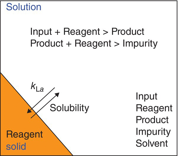
FIGURE 50.3 Representative process scheme for a solid–liquid reaction.
50.3.2.2 Mechanistic Studies
The next stage to build the model entails gathering mechanistic information for the kinetic and thermodynamic variables associated with the elementary steps. The goal of this stage is feeding the model with experimentally measured variables (e.g. reactant orders, rate and equilibrium constants, activation energies, solubility) to simplify and guide the subsequent numerical regression. For the elementary steps shown in Table 50.4, kinetic studies would afford reactant orders and initial values for rate constants (k), while temperature dependencies of the rate constants would provide activation energies (Ea) in agreement with the Arrhenius empirical equation (k = A exp[−Ea/RT]). Similarly, for reversible reactions, understanding the equilibrium expression and its position would afford the equilibrium constant (Keq) along with forward and reverse rate equations in thermodynamic consistency with equilibrium requirements (Table 50.5). Examination of the temperature dependence of the equilibrium constants would provide activation energies (Ea) in agreement with the van't Hoff equation (Keq = exp−ΔrHo/RTexpΔrSo/R).
TABLE 50.4 Rate Equations and Reaction Orders of Elementary Steps
| Elementary Step | Rate Equation | Reaction Order |
| A → P | Rate = k[A] | 1st |
| A + B → P | Rate = k[A][B] | 1st in A, 1st in B, 2nd overall |
| 2A → P | Rate = 2k[A]2 | 2nd |
| 2A + B → P | Rate = 2k[A]2[B] | 2nd in A, 1st in B, 3rd overall |
TABLE 50.5 Equilibrium Reaction with Forward and Reverse Rates
| Equilibrium | Requirement | Forward Rate | Reverse Rate |
| 2A ↔ P | Keq = [P]/[A]2 | Rate = ka[A]1.35 | Rate = kb[P]/[A]0.65 |
Mechanistic studies and elementary steps should be self‐consistent: e.g. an experimental rate law should concur with the proposed sequence of steps, and a kinetic isotope effect ought to match with the proposed rate‐limiting step in the sequence. In complex reactions, varying concentration–time curves due to changes in mechanism should be traceable to a common set of steps. Convoluted scenarios such as water‐sensitive transformations, autocatalysis or autoinhibition [15], catalyst deactivation [16], or mass transfer‐limited reactions [17] should be captured by the model, and their significance under different conditions ought to reflect the diverse kinetic profiles. Take, for example, the solid–liquid reaction shown in Figure 50.4. Simulation of mass transfer‐limited and non‐limited regimes in reagent (1.25 equiv. relative to input) maintaining k1 and k2 constant (k1/k2 = 50, Eqs. (50.4) and (50.5) affords distinct profiles that differ in the nature of the rate‐limiting step. Note that a simple 10‐fold increase in the mass transfer coefficient of the solid reagent shifts the rate‐limiting step from a mass transfer event (Eq. 50.3) to a chemical transformation (Eq. 50.4) and modifies conversion rates and curvatures for all components:
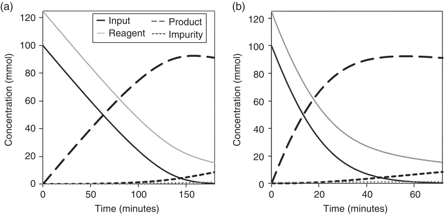
FIGURE 50.4 Concentration–time curves for a solid–liquid reaction under (a) mass transfer‐limited and (b) non‐limited regimes in reagent following 10‐fold increase in the mass transfer coefficient (see Figure 50.3 for the corresponding process scheme).
Since an account of the approaches used to conduct mechanistic studies falls beyond the scope of this chapter, secondary sources are selected in the references [18]. Traditionally perceived as resource intensive, mechanistic studies are currently facilitated by advancements of process analytical technologies (PAT) [12], parallel experimentation, and laboratory automation [19]. Collection of kinetic and thermodynamic knowledge can build on literature precedent and does not require recreation of the conditions used in the actual reaction step. For example, fast reactions can be slowed down at lower temperatures or higher dilutions to enable accurate rate measurements. Similarly, product degradation pathways leading to the formation of impurities can be studied in isolation from their direct precursors to maximize impurity levels and minimize experimental and analytical error.
50.3.2.3 Regression of Model Variables
Elementary steps and initial variables describe a preliminary model to which model‐building experiments run under representative process conditions will be regressed. The objective of this stage is to refine kinetic and thermodynamic variables characterized in the mechanistic studies and to regress the variables that were not experimentally measured. A DOE is completed to ensure that the model‐building data set covers the parameter space of interest. Parameters with potential impact on the QAs are chosen and their ranges selected to explore possible edges of failure based on existing knowledge. Typically, reaction aliquots are taken at intervals of adequate conversion and analyzed off‐line by HPLC to monitor the reactant and product concentrations, including impurities formed at low levels. The concentration–time data for each component are then introduced into the modeling software (e.g. DynoChem®)2 to numerically fit the experimental values until adequate convergence criteria are met (Figure 50.5).

FIGURE 50.5 Data and model fitting for impurity formation in representative model‐building experiment.
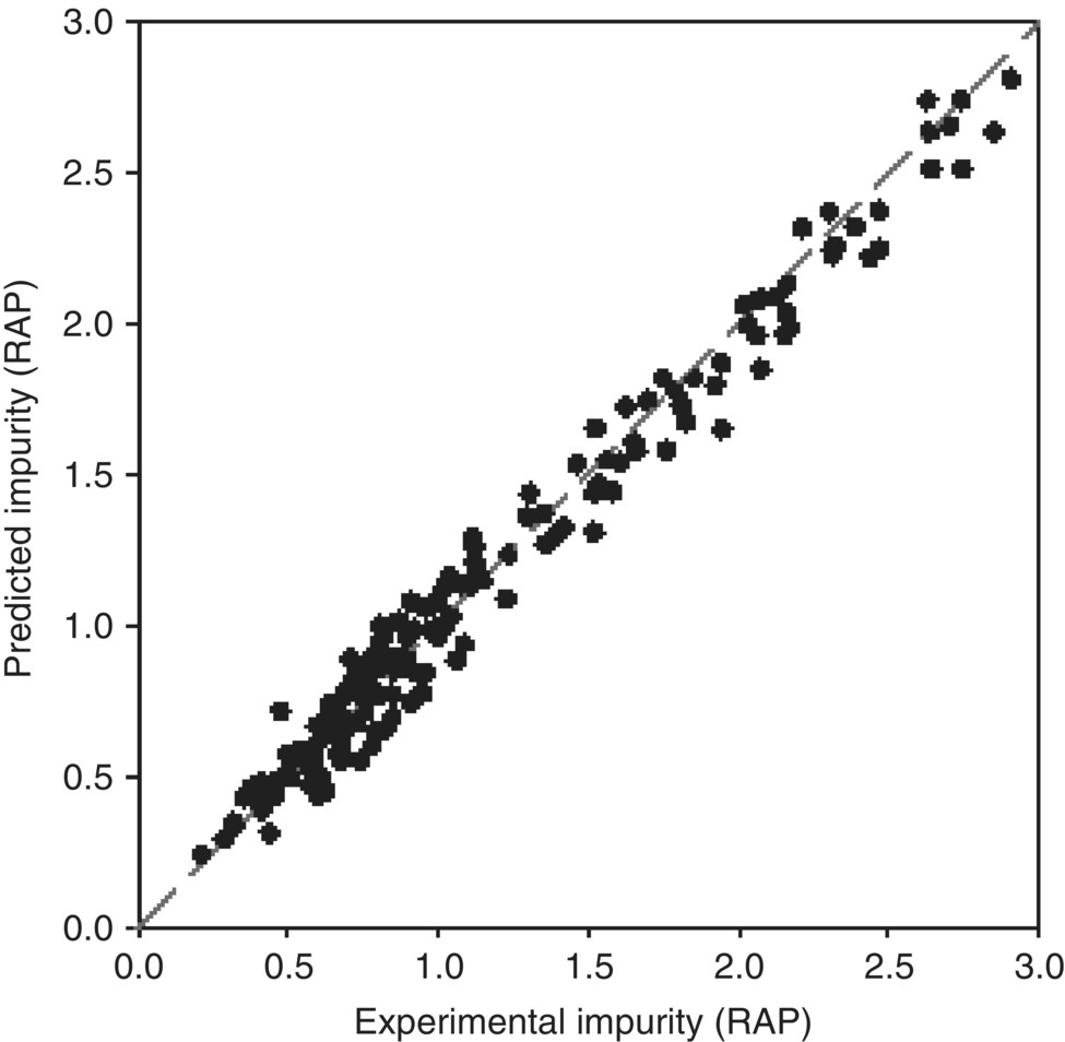
FIGURE 50.6 Parity plots for impurity formation in the model‐building experiments.
Source: From Ref. [23]. Reprinted with Permission. Copyright (2011) Springer Nature.
Acceptable fitting of experimental data to a model alone does not validate the predictive capability of the model. For example, overly complex models or models that regress an excessive number of variables relative to the size of the building data set may lead to overfitting and poor performance. A model overfits the building data set when it fits well this data set but has limited predictive power on an independent verification data set. Overfitting can be diagnosed via cross‐validation tests that split the building data set in subgroups for building and verification purposes. If overfitting occurs, iterative steps based on mechanistic information must be undertaken to mitigate the disconnection between model building and model verification. Poor performance due to model complexity can be addressed following simplification strategies such as network reduction [20], setting stoichiometric constraints [21], or applying the quasi‐equilibrium approximation when appropriate [22]. The regression of a disproportionate number of variables can be tackled by fixing them at values or ranges consistent with the mechanistic studies, and an inadequate sample size can be resolved by redefining the DOE. Alternatively, a model underfits the building data set when it does not capture the concentration–time data and shows biased trends. Underfitting is often due to oversimplified models that do not include the adequate elementary steps or satisfactory kinetic and thermodynamic variables. For example, underfitting occurs when a nonlinear rate dependence in a component is regressed to a linear dependence. The adjustment of a model that underfits cannot be achieved by revisiting the DOE. Instead, it demands an improved understanding of the origins of systematic error and a review of the mechanistic description of the reaction step.
50.3.2.4 Evaluation of Predictive Capability
With refined variables and a satisfactory fitting to the building data set, the predictive capability of the model can be evaluated by comparing its predictions against the experimental values measured in an independent verification data set. At this stage, laboratory experiments can be combined with plant batches to examine scale effects. Figure 50.7 shows superimposed parity plots of the model building and the verification data sets for impurity formation of a representative reaction (24 and 12 experiments, respectively, in HPLC relative area percent or RAP). A qualitative inspection of the plots suggests that the prediction errors are comparable for both sets across the range of impurity levels tested. Acceptable error magnitudes – e.g. root mean square error (RMSE) analysis affords no significant variation (<10%) in the prediction errors for the two data sets – and comparability between fitted and predicted impurity levels, including data at plant scale, indicate that the model is an adequate guide to develop a dependable design space at conditions and scales other than those used to build the model.
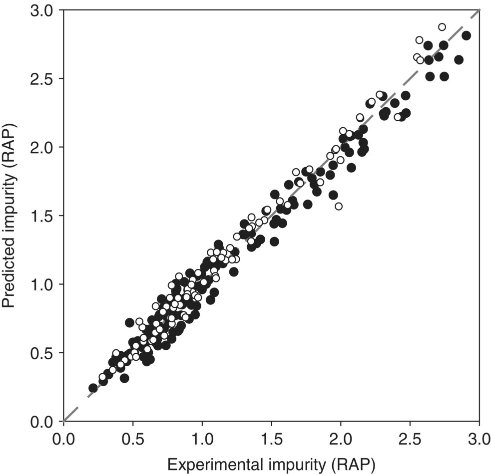
FIGURE 50.7 Parity plot of impurity formation for model‐building (○) and verification (●) data sets.
Source: From Ref. [23]. Reprinted with Permission. Copyright (2011) Springer Nature.
50.3.3 Development of an Empirical Model
Empirical models seek to correlate levels of significant species with MAs and process parameters by regressing a suitable, often low‐order polynomial that best describes the data set. The processes and variables considered in an empirical model do not rely on mechanistic information and are generally valid within the experimental space of interest in which the data set was collected. The development of a dependable model involves the following stages: (i) definition of the model's objective; (ii) selection of process parameters, parameter ranges, and levels; (iii) selection of the response variable; (iv) choice of experimental design; (v) performing the experiment; and (vi) statistical analysis of the data.
50.3.3.1 Defining the Objective
While outlining the objective of a predictive model is a critical step for both mechanistic and empirical approaches, the marked influence of the experimental design in the performance of empirical predictions requires a clear definition of the model's purpose [24]. If the objective is to elaborate a model that guides the space design selection, description of the functional relationship will proceed via an iterative scheme [25]. At the outset, preliminary experiments should target the identification and prioritization of the parameters that impact the reaction to narrow down the conditions where the eventual design space may reside. An exploratory screening can be carried out to cover a large parameter space with limited experimental burden at the expense of sacrificing model resolution by, for example, assuming linear responses. The screening could then be followed by optimization experiments to regress an improved model that adequately correlates the responses with process parameters. Graphical visualization of the functional relationship using three‐dimensional surface plots or two‐dimensional contour plots may prompt further revision of the empirical model or conclude that an appropriate relationship has been achieved. In contrast, if the goal is to explore process robustness within predetermined conditions (e.g. PARs), full iterative development of an empirical model is unnecessary, and the study of the functional relationship is limited to verifying a minimal or lack of response to parameter changes.
50.3.3.2 Selection of Process Parameters, Ranges, and Levels
Selection of the process parameters under scrutiny requires careful balance between the inclusion of a prohibitive number of parameters that may impact the reaction and neglecting parameters that may be critical to develop the functional relationship. An adequate choice relies on experimental information and scientific understanding. Risk assessment techniques used to prioritize the influence of process parameters often classify them into categories such as known to be impactful, suspected, possible, and unlikely. Reactant stoichiometries, concentration, and temperature are parameters examined routinely in reaction steps. Parameters not chosen for study can be held at a constant value or may be allowed to vary. For example, if extended reaction times lead to high levels of impurity, the experimental design can hold the reaction time constant at the highest value accepted for a commercial manufacturing setting, thereby representing the worst‐case scenario. In contrast, factors whose impact is very small within an anticipated range can be allowed to vary. For example, if multiple batches of input material have slightly different impurity profiles that are not expected to influence the results, a decision can be made to ignore batch variability and rely on randomization to balance out the effects that this difference could have.
Once the design parameters are selected, parameter variation ranges and specific levels at which the experiments will be carried out must be determined. Prior knowledge is often a good starting point. Early in model development, when the objective of experimentation is parameter screening, it is preferable to limit the number of levels to high and low. In general, the knowledge space is larger than the eventual design space, and, therefore, the range of parameter variation in this stage is broad. During the optimization phase, the two‐level design can be augmented to make the data set more suitable for model fitting. The ranges chosen for optimization must be relevant, achievable, and practical both from an experimental design and a commercial manufacturing perspective. Consideration of the plant capabilities where the process will be carried out in the long term is therefore an important aspect of parameter selection.
50.3.3.3 Selection of the Response Variable
Typical response variables selected for a reaction are yield, conversion, and level of the impurities that may impact the QAs of the step. Although several responses can be studied in a single DOE, it is important to search for unexpected responses. For example, if unknown impurities or unanticipated levels of known impurities result, further investigation is warranted to assess the impact of response variability upon quality.
50.3.3.4 Choice of Experimental Design
The distinct interconnection between model performance and experimental data demands a careful choice of the experimental design, which must consider data sets aligned with the objective of the model [26]. The design must provide a reasonable distribution of data points throughout the space of interest to ensure that the appropriate information can be collected and analyzed by statistical methods. It should allow for investigation of model adequacy, such as lack of fit, and provide a good profile of the prediction variance. Moreover, the design ought to facilitate the inclusion of follow‐up experiments needed to refine the model. For example, a two‐level factorial design adequate at the screening stage may need augmentation with center point replicates to estimate the experimental error. Similarly, a first‐order model that exhibits a lack of fit can be augmented by adding axial points to create a central composite design [27] or by including incomplete block designs [28] that lead to higher‐order terms in the fitting equation. Multiple types of experimental designs can be applied to the study of reactions, including computer‐generated optimal designs that are pertinent to special situations (e.g. irregular spaces of interest, nonstandard models, or costly experimentation). A detailed description of these designs is extensively discussed elsewhere [29].
50.3.3.5 Performing the Experiment
The execution planning of the actual experiments is often underestimated during the design stage. Performing a large number of experiments while pursuing accuracy and reproducibility to obtain meaningful results can be labor intensive. Modern high‐throughput and parallel automation tools can simplify the experimental setup and reduce material requirements by carrying out the reactions at milligram or gram scale. However, the implications of scaling down from commercial manufacturing conditions must be considered during model development. Furthermore, prior to conducting the experiment, a series of “familiarization” runs are recommended to probe reproducibility (e.g. triplicate experiments at the center point), obtain information about the consistency of the inputs and the measurement system, and provide an opportunity to practice the overall experimental technique.
50.3.3.6 Statistical Analysis of the Data
The results of the DOE are analyzed using statistical methods. Several software packages that can also be used in the experimental design are available to carry out the study. Initially, a combination of analysis of variance (ANOVA), post hoc tests, and graphical visualization will help identify the main effects of the significant variables and the interactions thereof. The experimental results are then regressed to fit an empirical model, that is, an equation derived from the data that expresses the relationship between the response and the important design parameters. Since the response variables (e.g. conversion, levels of impurity) follow an Arrhenius relationship, using a low‐order polynomial to fit the data may not be adequate. In these instances, variable transformation (e.g. using logarithm of time or inverse of temperature) can be employed to facilitate the polynomial fitting. Two techniques commonly used to help select the most relevant equation terms and improve predictive power are the forward stepwise regression and, more recently, genetic algorithms [11]. Forward step regression chooses the terms that offer the best response prediction and, sequentially, includes additional terms whose model coefficients are statistically significant. A genetic algorithm is a heuristic search that follows a defined set of rules to iteratively identify the subset terms that offer the best predictive power. The result of employing a genetic algorithm is a series of models that need further evaluation.
Completion of residual analysis and model adequacy checking helps to validate the appropriate mathematical model and provides guidance for additional follow‐up experimentation that could be required. A typical ANOVA and residual analysis using JMP® statistical software is shown in Figure 50.8. In this analysis report, an actual versus predicted plot (parity plot) provides a visual for the goodness of fit and the confidence curves for the model applied. Next, a summary of the model fit includes R2 (a measure of the variability of the response attributable to the regressor variables), ![]() (an adjusted form of R2 that helps guard against the inclusion of extra nonsignificant terms), and the RMSE (an estimate of the standard deviation of the random error). Following the summary of fit, the results of the ANOVA review the comparison of the fitted model against a model in which all the predicted values equal the mean response. The calculations of the sources of variance culminate in the F‐ratio (which analyzes the variance for the significance of regression) and the p‐value (which provides evidence that there is at least one significant effect in the model). The final sections display the parameter estimates for the regressed model (including p‐values for the individual parameters), a residual plot, and the final predictive equation (more appropriately described in Eq. (50.6)). Although the statistical analysis facilitates the initial validation of the model, its predictive power must be verified by testing the predictions for an independent data set not used in the regression of the model variables.
(an adjusted form of R2 that helps guard against the inclusion of extra nonsignificant terms), and the RMSE (an estimate of the standard deviation of the random error). Following the summary of fit, the results of the ANOVA review the comparison of the fitted model against a model in which all the predicted values equal the mean response. The calculations of the sources of variance culminate in the F‐ratio (which analyzes the variance for the significance of regression) and the p‐value (which provides evidence that there is at least one significant effect in the model). The final sections display the parameter estimates for the regressed model (including p‐values for the individual parameters), a residual plot, and the final predictive equation (more appropriately described in Eq. (50.6)). Although the statistical analysis facilitates the initial validation of the model, its predictive power must be verified by testing the predictions for an independent data set not used in the regression of the model variables.
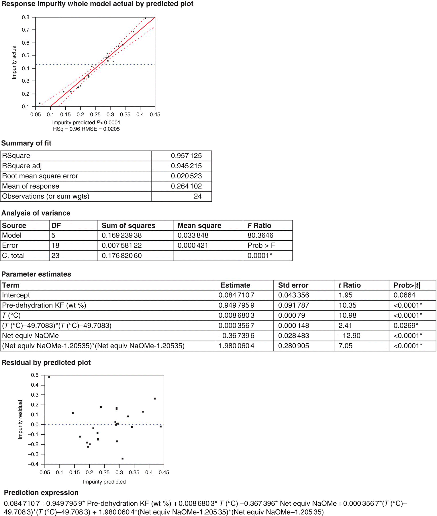
FIGURE 50.8 Representative example of ANOVA and residual analysis using JMP® statistical software.
Equation (50.6) – where A equals the initial KF values, B is the equivalents of NaOEt, T corresponds to the reaction temperature, and C equals the term (T − 49.8) – represents the analysis output that can be used to predict Impurity levels within the ranges and constraints considered in the building set:
50.4 DEFINING THE DESIGN SPACE
Translation of the process model, mechanistic or empirical, into a design space requires consideration of an approach that (i) can ensure drug substance quality, (ii) can be applied in routine manufacturing, and (iii) can be adequately presented to regulatory agencies for acceptance. This section outlines some of the most important considerations in developing and applying a model toward the definition of a design space.
50.4.1 Response Surfaces: Model Predictions and Impurity Level Contours
In the QbD paradigm, the terms knowledge space, design space, and operating space are used to describe the important processing regions where every parameter is a distinct dimension of a conceptual space (Figure 50.9). The knowledge space represents the region where the process is well understood by way of experiments, batch history, and empirical or mechanistic modeling, that is, operating at any combination of multiple parameters within this space has a predictable outcome. The design space consists of the region that has been demonstrated to assure quality product, and the operating space is the region targeted by the manufacturer for routine processing.
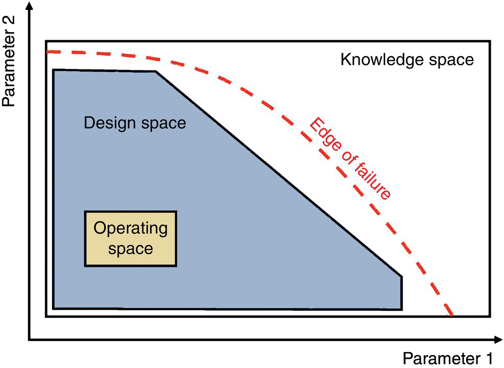
FIGURE 50.9 Illustration of a conventional knowledge, design, and operating space.
Once the model and the knowledge space where the model is valid are established, the goal of the practitioner is to define the design space, an inclusive subspace that considers the edges of failure and affords quality product at very high frequency. Additional laboratory experiments, pilot‐ or manufacturing‐scale batches, are often required to test the high risk regions and provide verification of quality product throughout the design space. Ultimately, the operating space is established by considering factory control capabilities, balance of efficiency (e.g. yield or cycle time), and high risk regions within the design space.
The most common approach to presenting and evaluating a model output is to compute response surfaces from the model equations with respect to two parameters. Figure 50.10 provides an example of a response surface, and Table 50.6 lists common parameters and responses evaluated in a reaction model. It is important to identify parameters that could be scale dependent, especially for multiphase reactions, to target a design that can be applied across scales. A response surface is also generally preferred by the regulatory agencies for presentation of the output of the model and justification of the design space. Several examples using response surfaces for presenting a design space are provided in the ICH Q8 (R2) Appendix [2].

FIGURE 50.10 Example of a response surface with respect to two parameters.
TABLE 50.6 Common Parameters and Responses Evaluated in a Reaction Model
| Common Reaction Parameters | Common Responses |
| Temperature profile | Impurity levels |
| Amount of starting material, reagents, product | Input conversion |
| Reaction volume | Yield |
| Reaction age | |
| Dosing rate | |
| kL a | |
| Agitation |
It is worth considering the enhancement in process knowledge gained through modeling compared with the traditional approach that defines PARs by testing one factor at a time. Figure 50.11 illustrates how PARs may fail to capture multivariate interactions between parameters in the context of response surfaces. While the operating conditions represented by point A are located within the PARs of Parameter 1 and Parameter 2, they lie beyond the edge of failure. Quality can be compromised if parameter interactions are not well understood and the operating conditions change for more than one parameter, even within their PARs.

FIGURE 50.11 Representation of an edge of failure in the context of PARs.
Multiple responses can be displayed together (e.g. yield, impurities, cycle time) by selectively shading or displaying specific contours. Visualization of the multiple responses affords a rich picture of the risks and benefits associated to operating at different points within the knowledge space. A limitation of response surfaces is that only two parameters can be displayed versus the response, whereas often the process requires to consider a conceptual space of higher order, i.e. n dimensions formed by n parameters – often termed as a hypercube for any space greater than three dimensions. The restriction may be overcome by either (i) reducing the discussion to the two parameters of highest impact in view of the practical variability or (ii) displaying multiple response surface plots to describe the higher‐order space. This approach will often display small projections of the design space by predicting the response surface at fixed, worst‐case, values for the parameters not included in the response surface graph.
50.4.2 Defining the In‐Process Limit for Impurities
The definition of a design space using response surfaces should consider contours that represent the edges of failure, that is, the limit for the response that ensures quality product. For a reaction model, each contour would commonly represent the in‐process limit of a given impurity. In‐process limits are determined from the drug substance specifications and fate and purge studies, which in turn may encompass several steps of the synthesis. Fate and purge studies often operate with intermediate limits and can include additional models to describe other unit operations.
50.4.3 Specifying and Presenting a Design Space in a Regulatory Submission
With a response surface and in‐process limits, a design space can now be defined. There are two general strategies to present a design space: (i) employing the entire mathematical model with n independent variables as a virtual n‐dimensional design space and dynamically determining, for each batch, the ranges of MAs and parameters that ensure quality and (ii) using the model predictions to select a subset projection of the space to define an invariant design space that can be represented by ranges of MAs and process parameters or a combination thereof [21]. To illustrate the two strategies, let us consider that all potential combinations of MAs and parameters defined by a mathematical model afford acceptable impurity levels in a tridimensional space characterized by the trapezoidal prism in Figure 50.12. A dynamic, model‐defined, approach could be chosen that provides access to all the parameter combinations within the prism. In contrast, an invariant approach would, for example, fix parameter z at its most conservative level, z1, and select the rectangular space represented by the small base of the prism. Whereas operating within the xy ranges denoted by this space would ensure success for all production batches, the invariant strategy provides access to only a subset of the parameter combinations. Allowing parameter z to change from z1 to z2 would expand the original projection to the rectangle represented by the large base of the prism. It is important to note that while in this example the invariant design space is shown as a two‐dimensional rectangle, there are several ways to express it. Design spaces could be specified through simple ranges that would form a square for two dimensions, a cube for three dimensions, or a hypercube for n > 3 dimensions. Alternatively, the parameters could be described in functions that afford a design space with irregular shape. Assigning a function to describe the edge of a design space can provide a wider operational space or enable access to a desired region. An example of a design space with a non‐cubic shape is provided in Section 50.5.2.

FIGURE 50.12 Representation of a hypothetical tridimensional trapezoidal prism operating space.
Although the dynamic strategy affords more flexibility, practical considerations have made the use of an invariant design space the method of choice for reaction steps. An essential requirement for a design space established through either approach is to verify that operating within the parametric region indeed ensures quality. This entails assessment against experimental data and verification across scales for application in a commercial process. A dynamic design space requires significant resources for rigorous model characterization and verification, as well as a long‐term commitment for model maintenance and revision. The importance of a model at ensuring product quality has implications on the level of detail in a regulatory submission, the degree to which the model should be assessed for fidelity, and its life‐cycle management. ICH provides a framework to categorize a model in low, medium, or high impact, depending on its importance to ensure quality [30]. Models used for design space selection are generally categorized as medium impact models. These models are expected to be described in detail with information pertaining to inputs, outputs, assumptions, and relevant equations. In the invariant approach case, a risk‐based, less resource‐intensive strategy can be used since the design space is a more constrained subset defined through parameter ranges. Furthermore, from an operational convenience perspective, a clear definition of ranges within which the production batches must always be carried out removes the need to dynamically calculate acceptable ranges for each batch by the manufacturing personnel.
50.5 VERIFICATION OF THE DESIGN SPACE
In a joined communication issued by the FDA and EMA, design space verification is defined as the demonstration that the proposed combination of input process parameters and MAs is capable of manufacturing quality product at commercial scale [31]. Verification is an experimental measure of performance directed to confirm that potential scale‐up effects or model assumptions are controlled within the design space limits and do not threaten the expected product quality. While it is possible to execute verification studies during process validation, design space verification should not be confused with process validation. Design space verification demonstrates adequate performance within the area of design space in relation to operations for which the space has been proposed. In contrast, process validation demonstrates consistency of the process at NORs and covers all the operations of the manufacturing process. Verification may occur over the life cycle of the product if changes within the design space pose unknown risks due to scale‐up effects.
50.5.1 Risk‐Based Approach to Design Space Verification
A risk‐based approach to design space verification for the final process prioritizes examination of the reaction step under worst‐case conditions. Since the limits of the design space are defined by specific ranges, not by model predictions, the model is simply used to guide the space selection, and the focus of the verification is the design space denoted by the parameter ranges rather than the model itself (Figure 50.13). Select experiments including replicates are run along the predicted edges of failure to independently explore the impact of process parameters and MAs at their high risk values. The experiments must be performed at a representative scale, and the reaction stream can be carried through the downstream operations chosen to isolate the product. For the verification to indicate that material of acceptable quality is generated throughout the design space, the isolated product has to meet the established specifications for all impurities and not just the impurity that may have been the focus of the design space development.
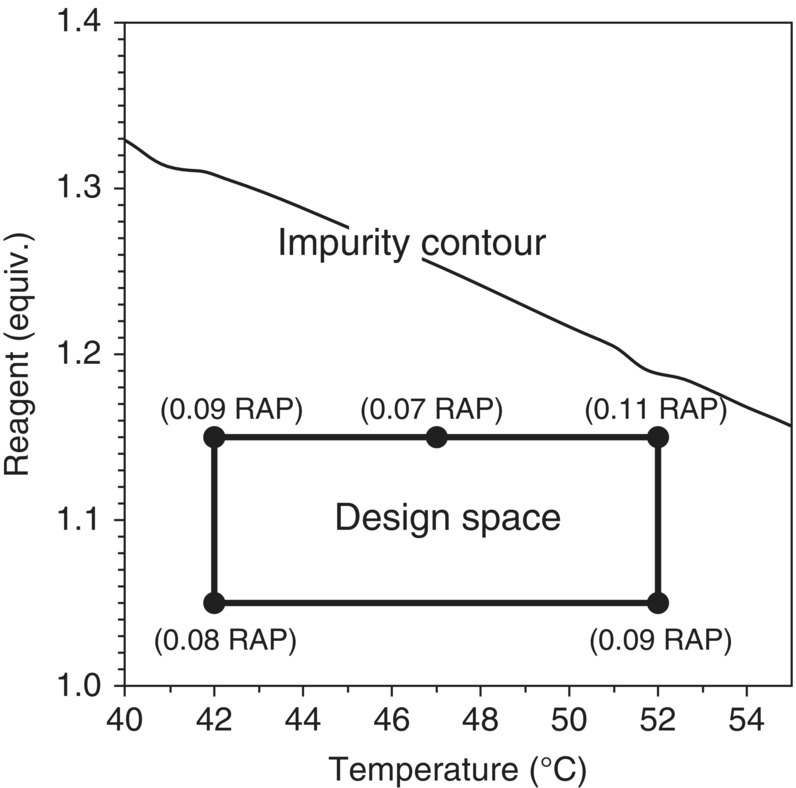
FIGURE 50.13 Representative design space verification. Numbers in parentheses represent impurity level (RAP) in isolated drug substance. The drug substance CQA limit for this impurity is less than or equal to 0.15%.
Source: From Ref. [23]. Reprinted with Permission. Copyright (2011) Springer Nature.
50.5.2 Relationship of Design Space to Scale and Equipment
A risk‐based approach can be applied to complete the design space verification prompted by changes on scale, equipment, or manufacturing site, since verification at commercial scale may not be possible. When a drug substance manufacturer demonstrates that a design space is scale independent, additional steps are not required for verification. However, changes within an unverified design space area that may pose risks due to scale‐up effects demand that these risks are understood and evaluated utilizing an appropriate control strategy. Scale independence can be justified based on scientific knowledge – including first principles, models, and equipment scale‐up factors [30, 32]. Ultimately, changes on scale or equipment require proper risk assessment and confirmation that the control strategy in place can deliver drug substance with acceptable quality.
For homogeneous reactions that have not shown scale or equipment limitations during development, scale and equipment independence can be confirmed by stressing multivariate experiments under worst‐case conditions of the proposed commercial equipment and demonstrating that the outcome matches design space predictions. Exploration of worst‐case conditions can entail the expansion of temperature ranges, simulation of heating or cooling profiles according to plant capabilities, or extension of the gap between laboratory and manufacturing reaction times. For heterogeneous or multiphasic reactions affected by mass transfer events, execution of laboratory simulations under worst‐case conditions must take place to demonstrate the lack of scale‐up effects on quality. For example, the anticipated role of scale and equipment upon mixing rates in a solid–liquid reaction can be deemed acceptable if product quality is not affected by particle size, agitation speed, or temporary loss of agitation under stressed experiments.
It is important to note that regulatory expectations about design space verification at commercial scale are not necessarily harmonized across health authorities [8] and that design space verification on commercial scale may be deemed indispensable to establish the commercial batch size. A protocol for design space verification based on a structured risk assessment has been reported in instances where adequate on‐scale data may not be available during filing [33]. This protocol considers initial design space verification, change management, and a specific reverification at commercial scale when changes within the design space relocate the process to areas of higher or unknown risk.
50.6 CASE STUDIES
The following case studies are provided to illustrate the construction of models for chemical reactions in API development and its application toward QbD for impurity control. The first and second case studies highlight two separate approaches for the same reaction. The first approach is an application of mechanistic modeling (Section 50.6.1), while the second approach is an application of empirical modeling (Section 50.6.2). These two case studies demonstrate that different strategies can be used to reach similar outcomes and allow a comparison of the advantages and disadvantages associated to each approach. The third case study is an application of mechanistic modeling to a much more complicated reaction (Section 50.6.3). It discusses a characteristic scenario including product degradation and the application of PAT to increase process robustness.
50.6.1 Mechanistic Model to Control a Critical Impurity in the Penultimate Step of a Drug Substance
This case study shows the development of a mechanistic model to control a critical impurity in the penultimate step of a drug substance [34]. The model contributes to the process design and control strategy by assisting in the selection and verification of the design space. This work was performed during the late‐stage process development of a drug substance and was used to provide an enhanced regulatory submission [35]. An impurity in the drug substance, Impurity B, was deemed critical after process development and risk assessment because it could impact the quality of the drug substance. Impurity B is formed from Impurity A, generated in the penultimate step reaction, and, therefore, also deemed critical (Figure 50.14). The final control strategy for Impurity B included the selection of a design space around the penultimate step reaction to control Impurity A to an acceptable in‐process level at reaction completion, which was established through fate and purge studies. The other major element of the control strategy was the specification for Impurity A in Final Intermediate (Table 50.7).

FIGURE 50.14 Ishikawa diagram for the Final Intermediate step.
Source: From Ref. [34]. Reprinted with Permission. Copyright (2010) Springer.
TABLE 50.7 Elements of Control Strategy for a Drug Substance
| Drug Substance Specifications | Type of Control | ||
| Procedural Controls | Material Attributes | Parameter Controls | |
| Impurity B NMT 0.15% | Crystallization of Final Intermediate and drug substance shown to purge Impurities A and B, respectively | In‐process controls: none Intermediate testing: Impurity A, NMT 1.0% in Final Intermediate |
Design space of the penultimate reaction to control Impurity A to NMT 1.76% post‐reaction |
The reactions of the penultimate step include the desired lactamization and an undesired lactam ethanolysis (Scheme 50.1 and Table 50.8). The lactamization of the Input material was divided in two steps: (i) a reversible deprotonation of the Input promoted by sodium ethoxide (NaOEt) and (ii) a first‐order rate‐limiting ring closure. The undesired ethanolysis occurs when NaOEt reacts with the product to open the lactam and afford the corresponding ethyl ester. During this reaction, the ethyl ester impurity exists as a salt that is later quenched with acetic acid to produce Impurity A. These transformations constitute a series of parallel reactions as NaOEt reacts with the Final Intermediate to generate the undesired impurity.
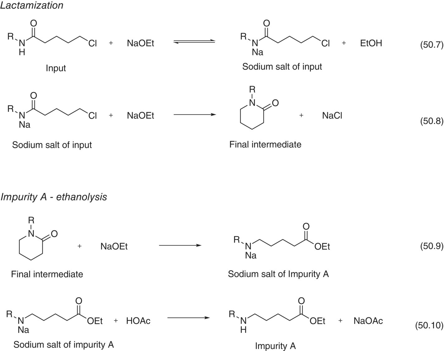
SCHEME 50.1 Formation of Final Intermediate and Impurity A.
Source: From Ref. [34]. Reprinted with Permission. Copyright (2010) Springer.
TABLE 50.8 Elementary Reactions of the Mechanistic Model
| Equation No. | Reaction | Chemical Equation |
| 50.7 | Deprotonation | Input + NaOEt ↔ Input‐Na salt + EtOH |
| 50.8 | Lactam ring closure | Input‐Na salt → Final Intermediate + NaCl |
| 50.9 | Ethanolysis | Final Intermediate + NaOEt → Impurity A‐Na salt |
Figure 50.15 shows the reaction profile of a representative experiment including the consumption of Input and the formation of Impurity A (Figure 50.15a and b, respectively) for one of the model‐building experiments (i.e. 1.25 equiv. NaOEt and 26°C). The reaction is typically completed in less than 1 hour, but aging past completion leads to additional growth of Impurity A. Extended reaction times are common for batch processes because additional time is taken to allow for a measurement of the reaction (e.g. HPLC analysis) to ensure completion before proceeding to the next unit operation. The inflection in the formation of Impurity A results from a procedural decrease in the reaction temperature implemented to help suppress the formation of Impurity A during the extended reaction time.

FIGURE 50.15 (a) Concentration–time curves and model fitting for the consumption of Input (◊) and formation of Impurity A (○). (b) Rescaled version of Figure 50.15a to display Impurity A.
Source: From Ref. [34]. Reprinted with Permission. Copyright (2010) Springer.
Preliminary studies indicated that temperature and excess NaOEt were the parameters with the highest impact to the formation of Impurity A. Consequently, a central composite design with 10 experiments was conducted across the space of interest to generate the model‐building data set for parameter regression (Figure 50.16). It is worth mentioning that NaOEt charges were made in an ethanol solution and that changes in excess NaOEt inflicted variations in other parameters known to impact the reaction, such as concentration and solvent composition.
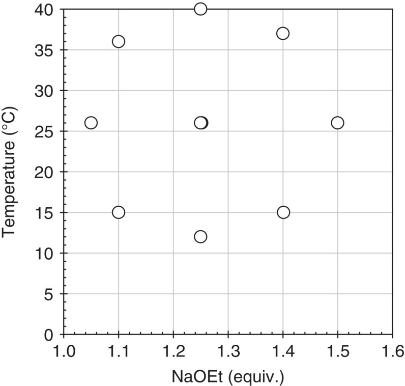
FIGURE 50.16 Graphical representation of the experimental conditions for the model‐building set.
Source: From Ref. [34]. Reprinted with Permission. Copyright (2010) Springer.
The reaction constants, activation energies, and equilibrium constant for the deprotonation of the Input were regressed using DynoChem® modeling software [20] (Table 50.9). Figure 50.17 shows concentration–time curves for Impurity A and associated model fitting for 12 experiments of the model‐building set, which included changes in the excess NaOEt (1.05–1.50 equiv.) and temperature (12–40 °C). Note that an imposed temperature profile consisting of the reaction temperature and a cooling ramp to suppress reaction progress during analytical testing was applied to mimic the intended manufacturing procedure. Profiles represented by solid curves result from fitting the data to the mechanistic model under the corresponding reaction conditions. The differential equations based on the rate expression and the regressed variables provided a model that could be used to predict the consumption of Input and the formation of Impurity A with respect to temperature profile, reaction time, concentration of Input, and equivalents of NaOEt.
TABLE 50.9 Rate Expressions and Regressed Model Variables
| Equation No. | Reaction | Rate Expression | ka (l/mol.min) | Ea (kJ/mol) | Keq a |
| 50.7 | Deprotonation | rd = kd [Input][NaOEt] | 161.3 (19%)b | 26.6 (41%)b | 1.54 (65%)b |
| 50.8 | Lactam ring closure | r1 = k1 [Input‐Na salt] | 0.0194c (38%)b | 87.0 (13%)b | — |
| 50.9 | Ethanolysis | re = ke [Final Intermediate][NaOEt] | 0.0027 (2.9%)b | 81.9 (4%)b | — |
aTref = 25 °C.
b95% confidence interval.
ck value in 1/s units.

FIGURE 50.17 Concentration–time curves and model fitting for the formation of Impurity A (○) for the 12 model‐building experiments varying NaOEt equiv. and temperature: (a) 1.10 equiv., 15°C; (b) 1.05 equiv., 26°C; (c) 1.25 equiv., 12°C; (d) 1.40 equiv., 15°C; (e) 1.10 equiv., 36°C; (f) 1.25 equiv., 26°C; (g) 1.25 equiv., 26°C; (h) 1.25 equiv., 26°C; (i) 1.25 equiv., 26°C; (j) 1.50 equiv., 26°C; (k) 1.25 equiv., 40°C; and (l) 1.40 equiv., 37°C.
Source: From Ref. [34]. Reprinted with Permission. Copyright (2010) Springer.
The predictive capability of the model was assessed by comparing the predicted versus experimental levels of Impurity A for model‐building and verification data sets in a parity plot and by quantitative error analysis for each data set (Figure 50.18 and Table 50.10, respectively). The assessment consisted of nine lab‐scale experiments and five manufacturing‐scale batches that were not included in the model regression. The strong agreement between the model‐building set and the verification set demonstrates the high fidelity of the model and the independence of scale, which was expected for this liquid‐phase homogeneous reaction.
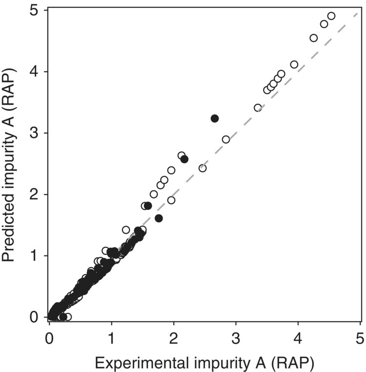
FIGURE 50.18 Parity plot of Impurity A formation for the model‐building (○) and verification (●) data sets.
Source: From Ref. [34]. Reprinted with Permission. Copyright (2010) Springer.
TABLE 50.10 Quantitative Error Analysis for Model‐Building and Model Verification Data Sets
Source: From Ref. [34].
| Model‐Building Set | Model Verification Set | |
| RMSE (RAP) | 0.16 | 0.13 |
| Mean relative error (%) | 11.2 | 10.6 |
| Maximum absolute error (RAP) | 0.51 | 0.40 |
Despite the high accuracy of the model, the elementary equations in Table 50.8 represent a simplified system that does not capture all of the chemical interactions. For instance, it was found that the ethanol to N‐methylpyrrolidone solvent ratio significantly impacts the ethanolysis reaction. This parameter was considered intractable for inclusion in the model but was captured by determining acceptable ranges and holding it at a constant worst‐case value in relation to impurity formation. This approach simplified model development while accounting for the influence of solvent composition.
To determine the parameter ranges that would constitute the design space, response surfaces were generated for consumption of Input at the time of reaction sampling and levels of Impurity A upon reaction quench with respect to temperature and excess NaOEt (Figure 50.19). The response surfaces represent the computational prediction of the concentration of Input and Impurity A across the parameter ranges and initial conditions simulated in the virtual experiments. Moreover, it was necessary to define values for other parameters that affected the levels of Impurity A (Table 50.11). These parameters were varied in the model‐building experiments and shown to influence model prediction but were less impactful than temperature and excess NaOEt. The values of these less impactful parameters were chosen within predefined ranges that would afford the highest level of Impurity A, thereby providing the most conservative projection of the edges of failure.
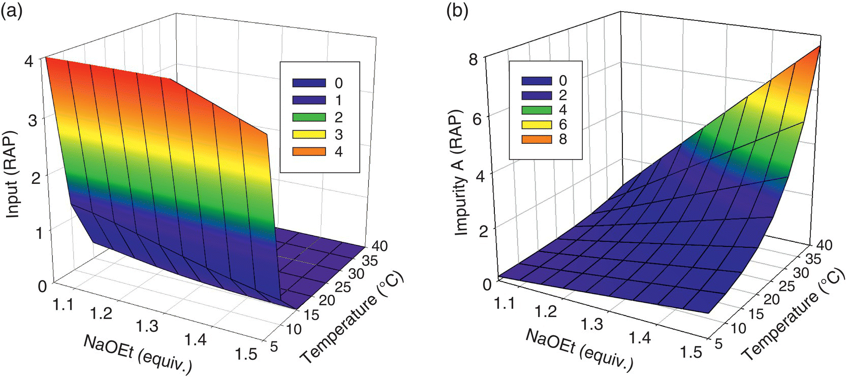
FIGURE 50.19 Response surfaces for (a) residual levels of input and (b) levels of Impurity A.
Source: From Ref. [34]. Reprinted with Permission. Copyright (2010) Springer.
TABLE 50.11 Conservative Values of the Process Parameters for the Lactamization
| Conservative Values | ||
| Process Parameter | Minimum | Maximum |
| Substrate concentration | 8.9 wt % | |
| Reaction age time | 60 min | |
| Total reaction age time above hold temperature | 180 min | |
| Reaction hold temperature | 10 °C | |
The response surfaces were displayed as contour plots to visualize the desired and undesired regions of operation. Figure 50.20 shows how low temperatures should be avoided to ensure reaction completion and minimize residual Input plots at the time of reaction sampling, while high temperatures and high equivalents of NaOEt should be avoided to minimize the levels of Impurity A upon reaction quench. The acceptable operating region was resolved by combining Figure 50.20a and b and displaying the contours of interest, that is, the acceptable in‐process levels for Input and Impurity A (Figure 50.21).
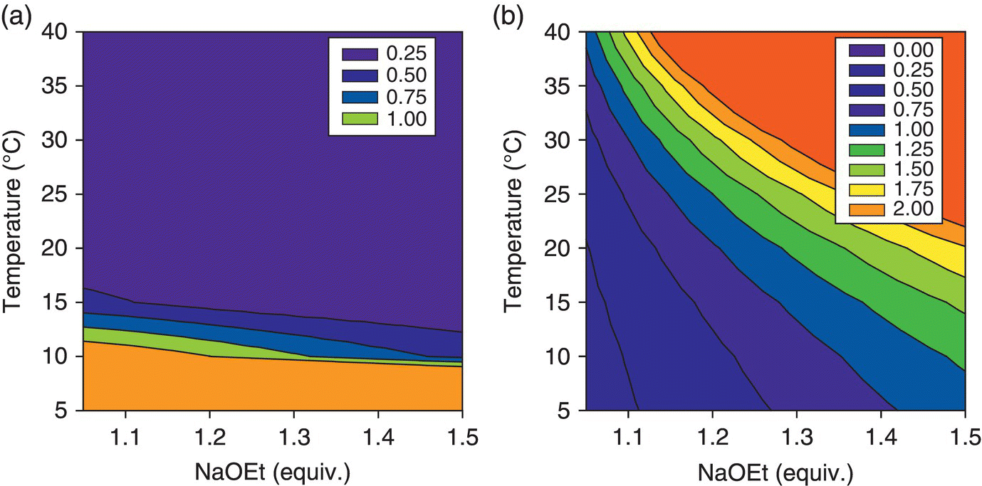
FIGURE 50.20 Contour plots of the response surface for (a) residual levels of Input and (b) levels of Impurity A.
Source: From Ref. [34]. Reprinted with Permission. Copyright (2010) Springer.
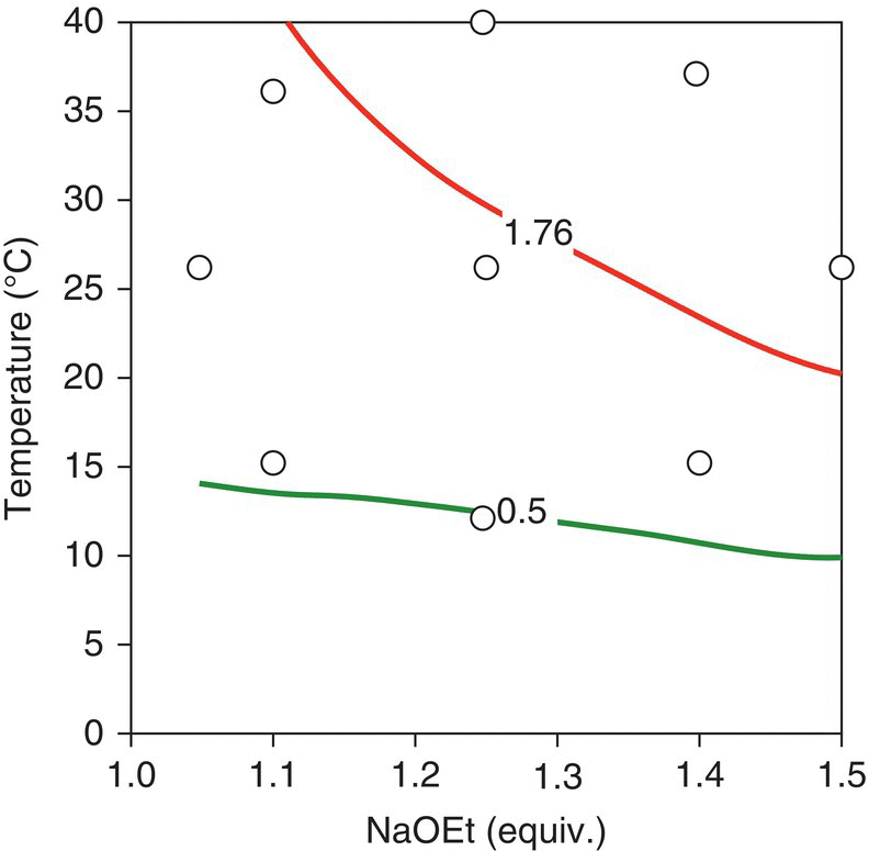
FIGURE 50.21 Combined contour plots including the contour of 1.76 RAP for residual levels of Input (lower line) and the contour of 0.5 RAP for levels of Impurity A (upper line). Location of the model‐building experiments (○) is shown to illustrate that the calibration set spans within and beyond the desired operating region.
Source: From Ref. [34]. Reprinted with Permission. Copyright (2010) Springer.
Guided by these conservative response surfaces, the final design space was selected as a trapezoidal region between the edges of failure for residual input and Impurity A (Figure 50.22). This design space was described by a temperature range of 15–30 °C, a NaOEt range of 1.1–1.4 equiv., and an equation for the edge of the trapezoid, T = −70B + 113, where T is the temperature in °C and B is the excess NaOEt in equivalents. Design space verification was carried out by conducting a set of experiments at the extreme points of the trapezoid and taking the reaction to the isolated Final Intermediate for analysis using the release method. Table 50.12 displays the results of these experiments, including predicted and experimental in‐process levels of Impurity A, and the value of Impurity A in isolated cake. The model showed strong performance for the prediction of Impurity A at the same time that the Final Intermediate met the specification for Impurity A (NMT 1.0%). Based on these results, there was high confidence that the design space selected would provide a robustness element in the overall control strategy for Impurity A.

FIGURE 50.22 Trapezoidal design space. Results of verification experiments are given in parenthesis for in‐process and isolated cake levels of Impurity A, respectively.
Source: From Ref. [34]. Reprinted with Permission. Copyright (2010) Springer.
TABLE 50.12 Results of Verification Experiments for In‐Process and Isolated Cake Levels of Impurity A
| NaOEt (equiv.) | Temperature (°C) | Impurity A In‐Process Model Prediction (RAP) | Impurity A In‐Process Experimental (RAP) | Impurity A Isolated Cake Value (RAP) |
| 1.10 | 15 | 0.32 | 0.39 | 0.27 |
| 1.10 | 30 | 0.80 | 0.93 | 0.58 |
| 1.40 | 15 | 1.08 | 0.91 | 0.53 |
| 1.19 | 30 | 1.41 | 1.43 | 0.84 |
| 1.25 | 26 | 1.41 | 1.50 | 0.85 |
| 1.25 | 26 | 1.33 | 1.47 | 0.83 |
| 1.25 | 26 | 1.36 | 1.44 | 0.78 |
| 1.25 | 26 | 1.32 | 1.38 | 0.76 |
Given that any model is a simplified representation of the actual system and that the experimental measurements and the regression have inherent uncertainty, the predicted edges of failure had some uncertainty. Rather than attempting to calculate the uncertainty about the edge of failure, the variability around the design space with respect to failure was assessed. For this analysis, multiple experiments were conducted in the highest risk region, and the variability around this point was determined. Table 50.12 shows the results of experiments conducted at 26 °C and 1.25 equiv. of NaOEt, and Table 50.13 shows the calculation of the variability at this point. The distribution of in‐process and isolated cake impurity levels showed that the mean in‐process level and dry cake level were 1.45 and 0.81, respectively. Furthermore, the upper tolerance limit (95% confidence and 90% proportion) for the in‐process and isolated cake distribution was 1.67 and 0.99. The tolerance limit for both in‐process and isolated cake was within the specifications levels established, that is, 1.76 AP RAP and 1.0 RAP, respectively.
TABLE 50.13 Variability of Experiments Conducted at 26 °C and 1.25 equiv. of NaOEt
| Impurity A In‐Process RAP | Impurity A Isolated Cake RAP | |
| Mean | 1.45 | 0.81 |
| Standard deviation | 0.054 | 0.044 |
| Upper tolerance limit | ||
| (1‐alpha = 0.95, proportion = 0.90) | 1.67 | 0.99 |
This design space was verified to reproducibly deliver product of acceptable quality at all locations, including the highest risk regions. It was accepted by regulatory agencies as reported in the drug master file and, most importantly, supported the manufacture of a drug substance that has been routinely made during several years without off‐specification results for Impurity B in the drug substance. A deep level of knowledge was obtained that shaped the final design of the process through building the mechanistic model. Procedural changes, such as cooling the batch after a prescribed reaction time or controlling the exotherm through different NaOEt addition profiles, could be quickly assessed by running virtual experiments and implemented based on fundamental knowledge.
50.6.2 Empirical Model to Control a Critical Impurity in the Penultimate Step of a Drug Substance
This case study is an extension of the case study presented in Section 50.5.1 wherein, instead of a mechanistic model, an empirical model was employed to investigate the selection of a design space to control Impurity A. The same overall control strategy (Table 50.7) and reactions (Scheme 50.1) are relevant to building the empirical model, but rather than determining the mechanism and rate expression for the reaction, a polynomial expression of the statically significant factors was used to predict the edge of failure. In addition, the reaction procedure and target completion value were identical as described in Section 50.5.1. This study demonstrates that the empirical approach can achieve a satisfactory outcome and highlights some of its advantages and disadvantages relative to the mechanistic approach.
A central composite experimental design was conducted with the intention to build either a mechanistic or empirical model (Figure 50.16). The DOE consisted of a full‐factorial, two‐factor, and two‐level design with four center points and four additional axial points to facilitate the accurate prediction of the curvature of the response. The two factors considered were reaction temperature and equivalents of NaOEt. The response measured in the DOE was the final level of Impurity A prior to quenching the reaction, which includes the extended reaction time required for in‐process control analysis of reaction completion. The analysis of the DOE data was performed using JMP® statistical software package, including the generation of a model that considered first‐ and second‐order effects as well as potential interactions between temperature and the equivalents of NaOEt. The JMP® output provided (i) the ANOVA, which tests the hypothesis that parameter terms are zero with exception of the intercept; (ii) the lack of fit, which assesses whether the model fits the data well; and (iii) parameter estimates for the significant factors that define the empirical model. Equation (50.11), where B equals the equivalents of NaOEt and T equals the temperature of the reaction, is the final output of this analysis and can be applied to predict levels of Impurity A within the ranges of the data set and the procedural constraints applied in the model‐building set. Analysis tables of primary interest shown in Figure 50.23 indicate that all the parameter estimates are statistically significant and support a good model fit as shown by the high R2 value and low RMSE:
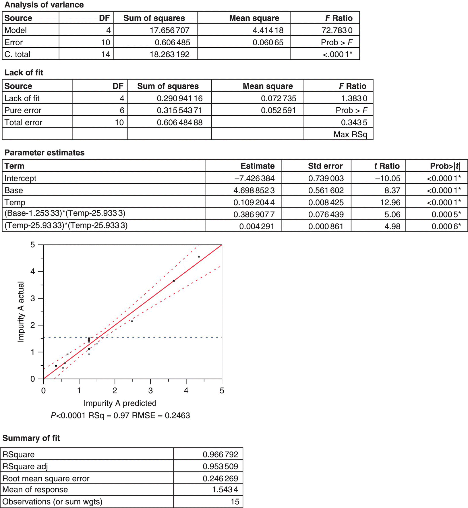
FIGURE 50.23 Representative ANOVA and residual analysis using JMP® statistical software.
Similar to the mechanistic model analysis, a parity plot can provide a qualitative assessment of the model fit (Figure 50.24).

FIGURE 50.24 Parity plot of Impurity A formation for the model‐building (○) and verification (●) data sets.
Source: From Ref. [34]. Reprinted with Permission. Copyright (2010) Springer.
The empirical model was used to predict the contour of the 1.76 RAP in‐process specification for Impurity A. Figure 50.25 compares contours predicted with both the empirical and the mechanistic models. Interestingly, the mechanistic and empirical models show nearly identical predictions for the edge of failure, indicating that both approaches can guide the selection of the design space below the edge of failure and ultimately define the trapezoidal space shown in Figure 50.22.

FIGURE 50.25 (a) Response surface for levels of Impurity A predicted by the empirical model. (b) Empirical (‐‐‐) and mechanistic (—) model predictions for the edge of failure.
Source: From Ref. [34]. Reprinted with Permission. Copyright (2010) Springer.
As expected, the empirical approach was more efficient than the mechanistic approach from an experimental and computational perspective. Overall, the empirical approach involved a more simplistic tactic where no consideration of the reaction mechanism was required. Moreover, the model provided an equation that was easily described and presented. However, while the mechanistic model required much more consideration of the underlying physical organic principles and additional experiments to confirm the mechanistic hypothesis, this effort provided its primary benefit and in‐depth understanding of the reaction. In many cases fundamental knowledge can be leveraged to improve the process and provide a more efficient or robust design. For instance, in this case study, the effect of cooling the reaction after a defined reaction age to reduce impurity formation during analytical testing could be easily explored with the mechanistic model. In contrast, the empirical model was valid for a very specific procedure and could not predict deviations regarding the timing of the operations or alternative profiles of variant parameters such as temperature. This could be a limitation as the scale of the reaction increases. For example, while the dosing profile of NaOEt produces an exotherm that results in a minor increase in temperature at the laboratory scale, if the manufacturing scale provided a different degree of heat removal or the dosing profile was altered slightly, the temperature profile could be altered. Although the design space could still be valid, the empirical model would not be able to provide an accurate prediction.
The practitioner must first weigh the complexity of building a mechanistic model and the importance of fundamental understanding against the efficiency and expedience gained through an empirical approach. Careful consideration of the procedural constraints and the variant parameters must be considered in either approach but especially if an empirical approach is taken.
50.6.3 Mechanistic Model and Role of PAT in the Penultimate Step of a Drug Substance
Selection of the design space for the Final Intermediate step of a drug substance was guided by a mechanistic model [36]. Preparation of the Final Intermediate entailed the condensation of a heteroaryl halide (Input 1) with a highly functionalized starting material (Input 2). The transformation involved (i) deprotonation of Input 2 with potassium tert‐butoxide (t‐BuOK) to form a tripotassium salt (Compound 1) that was not isolated, (ii) condensation between the heteroaryl halide and the alkoxide group of Compound 1 to form Compound 2 as its salt, and (iii) aqueous quench upon reaction completion. The Final Intermediate would be obtained following workup, crystallization, isolation, and drying operations.
A collective risk assessment of the drug substance CQAs and a process risk assessment of the parameters affecting the step identified the Final Intermediate QAs as assay, identity, and impurities. Six process‐related impurities were studied (i.e. impurities A–F), but only two were critical to quality and yield (impurities A and B, respectively). Impurity B is the major impurity generated in the reaction, but it purges to a high degree during the crystallization. In contrast, Impurity A is of high interest due to its lower purging in the subsequent operations and its capability to lead to an impurity that may impact drug substance quality. The levels of impurities C–F remained within the purging capability of the process. The simplified Ishikawa diagram shown in Figure 50.26 depicts the step with regard to the QAs of the Final Intermediate.

FIGURE 50.26 Ishikawa diagram for the Final Intermediate step.
Source: From Ref. [36]. Reprinted with Permission. Copyright (2016) American Chemical Society.
Reaction conditions that would enable the control of impurities A and B within acceptable limits were evaluated by means of a mechanistic model. Construction of the model began with kinetic studies to understand Final Intermediate formation, consumption of input materials, and the generation of impurities. The knowledge thus gathered was used to articulate the elementary reactions described in Table 50.14. As shown in Scheme 50.2, condensation of Input 1 (the electrophile) and Compound 1 (the nucleophilic tripotassium salt of Input 2) affords Compound 2, the dipotassium salt that forms Final Intermediate upon aqueous quench. Deprotonation of Input 2 by addition of greater than 3 equiv. of t‐BuOK was demonstrated to be complete and instantaneous under studied temperatures, and, consequently, the model approximates the initial concentration of Compound 1 with the concentration of its precursor Input 2.
TABLE 50.14 Elementary Reactions of the Mechanistic Model
Source: From Ref. [34].
| Equation No. | Reaction | Chemical Equation |
| 50.17 | Reaction of base with water | t‐BuOK + H2O → KOH + t‐BuOH |
| 50.12 | Formation of Final Intermediate | Compound 1 + Input 1 → Compound 2 + KCl |
| 50.18 | Final Intermediate equilibrium | Compound 2 ↔ Transient Species I + t‐BuOK |
| 50.13 | Formation of Impurity A | Transient Species I + Compound 1 → Impurity A |
| 50.14 | Formation of Impurity B (hydrolysis) | Input 1 + KOH → Impurity B Intermediate + KCl |
| 50.15 | Formation of Impurity B (hydrolysis) | Impurity B Intermediate + t‐BuOK → Impurity B + t‐BuOH |
| 50.16 | Formation of Impurities B and C (β‐elimination) | Compound 2 + t‐BuOK → Impurity B + Impurity C + t‐BuOH |
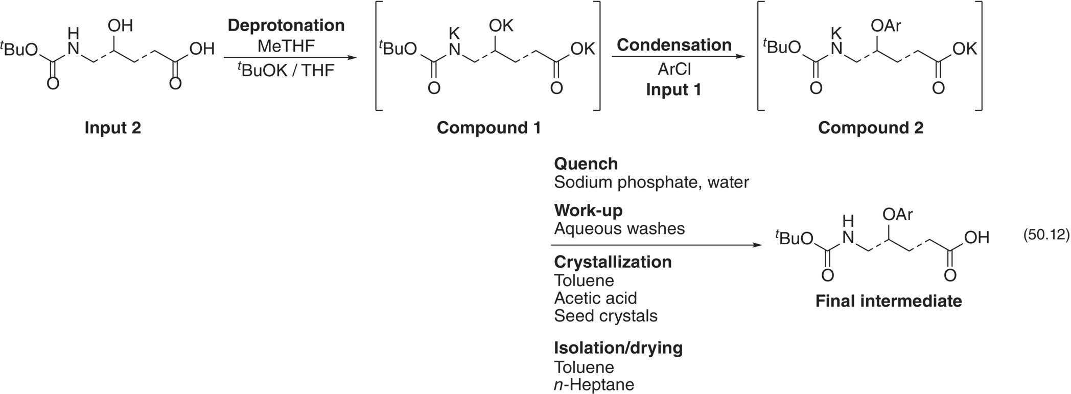
SCHEME 50.2 Preparation of the Final Intermediate.
Source: From Ref. [36]. Reprinted with Permission. Copyright (2016) American Chemical Society.
Impurity A is generated by addition of unreacted Compound 1 to a transient species derived from Compound 2, which in turn is in equilibrium with Impurity A (Eq. (50.13), Scheme 50.3) [37]. The concentration of Impurity A depends on the ratio of Compound 2 to t‐BuOK since both nucleophiles compete for the transient intermediate. In agreement with this observation, the reaction that forms Impurity A displays an inverse‐order dependence on the t‐BuOK concentration. On the other hand, Impurity B is formed via two pathways, fast hydrolysis of Input 1 (Eq. 50.14) and slow degradation of the desired product through β‐elimination promoted by t‐BuOK (Eq. 50.15). Accordingly, the growth of impurity B shows a bimodal kinetic profile with a rapid onset followed by a slow progression. Superimposition of the inhibitory effect of t‐BuOK concentrations upon the levels of Impurity A and the promoting effect of t‐BuOK concentrations upon the levels of Impurity B explains why controlling the charge of base is crucial. Low excess base affords higher levels of Impurity A, whereas high excess base leads to decomposition of Compound 2 by β‐elimination, resulting in higher levels of Impurity B.
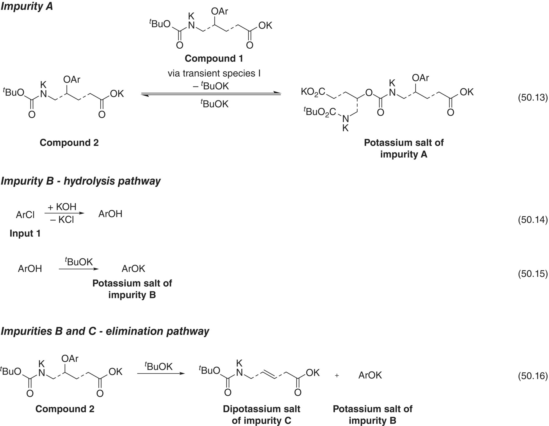
SCHEME 50.3 Formation of Impurities A and B. Equations 50.17 and 50.18 in Table 50.14 are not shown for simplification.
Source: From Ref. [36]. Reprinted with Permission. Copyright (2016) American Chemical Society.
Although Impurities C–F were always generated within the purging capability of the process and did not affect the quality of the Final Intermediate, they were incorporated in the mechanistic model because their formation influences the concentrations of the main reaction components, including impurities A and B. For example, Impurity C is formed during the β‐elimination pathway that generates Impurity B and contributes to the consumption of t‐BuOK (Eq. 50.16).
Since the reaction mixture formed a slurry comprising Compounds 1 and 2, the solubility of the two salts was investigated. The solubility of Compound 1 was nearly constant within the studied temperature range, whereas the solubility of Compound 2 showed a marked dependence on temperature. The van't Hoff equation [38] was used to correlate the experimental solubility of Compound 2 with temperature, and the solubility equilibria for Compounds 1 and 2 were incorporated into the mechanistic model (Table 50.15).
TABLE 50.15 Solubility of Compounds 1 and 2
| Species | Solubility | ln(As) | Bs (kJ/mol) |
| Compound 1 | 0.06 mol/l | — | — |
| Compound 2 | Solubility (mg/ml) = As·e(Bs/RT) | 10.53 | 17.80 |
The van't Hoff equation defines the logarithm of solute concentration as a linear function of the reciprocal of absolute temperature; variables A and B were calculated using a least squares analysis.
Model variables for the elementary reactions were regressed using a series of model‐building experiments. In these experiments, process parameters with a high impact on the formation of Impurities A and B were varied to comprise the likely design ranges and to explore potential edges of failure based on existing knowledge. A total of 10 reactions were conducted using a central composite design with 2 center points to assess reproducibility. The excess equivalents of base were varied from 0.05 to 1.0 equiv. and the temperature from 40 to 65 °C. The amount of Input 2, solvent, water from Inputs, and reaction time were also varied. Over the course of the reactions, the concentrations of Input 1, Input 2, Final Intermediate, and Impurities A–F were measured by HPLC analysis of sample aliquots (10–15 per experiment), introduced into the DynoChem® modeling software21, and used to fit their values until adequate convergence criteria were met. Rate expressions for elementary reactions and regressed model variables are shown in Table 50.16.
TABLE 50.16 Rate Expressions and Regressed Model Variables
| Equation No. | Reaction | Rate Expression | k (l/mol·min) | Ea (kJ/mol) | Keq x 103 (1/s) |
| 50.17 | Reaction of base with water | r = k[t‐BuOK] [H2O] | 1 × 10² | 20 | — |
| 50.12 | Formation of Final Intermediate | r = k[Compound 1][Input 1] | 6.48 × 10⁻³ | 84.6 | — |
| 50.18 | Final Intermediate equilibrium | rf = k[Compound 2] r = k [Transient Species I] [t‐BuOK] |
8.97 1/s | 11.3 53.4 |
0.54 |
| 50.13 | Formation of Impurity A | r = k[Transient Species I][Compound1] | 4.59 × 10⁻⁴ | 160.6 | |
| 50.14 | Formation of Impurity B (hydrolysis) | r = k[Input 1][KOH] | 1.53 × 10⁻² | 5.7 | |
| 50.15 | Formation of Impurity B (hydrolysis) | r = k[Impurity B Intermediate][ t‐BuOK] | 16.7 | 16.2 | — |
| 50.16 | Formation of Impurities B and C (β‐elimination) | r = k[Compound 2][t‐BuOK] | 6.21 × 10⁻⁵ | 97.0 | — |
Representative plots for the decay of Input 2, formation of Final Intermediate, and growth of Impurities A and B are shown in Figure 50.27. Fitting the experimental data to the reaction conditions affords the profiles shown in dashed curves. Concentrations of Final Intermediate decrease at extended reaction times mainly due to the formation of Impurity B. The growth of Impurity B displays a bimodal profile: its initial progress is dictated by the hydrolysis of Input 1 promoted by water in the Input materials (Equations (50.14) and (50.15), Scheme 50.3), and, as the reaction proceeds, it forms at slower rates caused by β‐elimination of the Final Intermediate in the presence of excess base (Equation (50.16), Scheme 50.3).

FIGURE 50.27 Concentration–time curves and model fitting for (a) consumption of Input 2 and formation of Final Intermediate and (b) growth of impurities A and B for the same reaction. The experimental data corresponds to a reaction performed at 45 °C with 0.80 equiv. of excess t‐BuOK.
Source: From Ref. [36]. Reprinted with Permission. Copyright (2016) American Chemical Society.

FIGURE 50.28 Parity plots of the model verification and building data sets for (a) Impurity A and (b) Impurity B.
Source: From Ref. [36]. Reprinted with Permission. Copyright (2016) American Chemical Society.
The predictive capability of the model was evaluated by comparing its predictions against the values measured in a series of verification experiments. Figure 50.27 shows parity plots of the model‐building data set and the verification data set for Impurities A and B. The verification data set consisted of six reactions at laboratory scale and eight batches at pilot plant scale. A RMSE analysis of the parity plots shows that the prediction errors in the model‐building data set and the verification data set are comparable across the range of impurity levels tested (RMSE ˂ 10%). Acceptable error magnitudes and comparability between fitted and predicted impurity levels indicated that the model is an adequate guide to develop a dependable design space.
Specifications for impurities A and B in the isolated Final Intermediate needed to be first established and then correlated with in‐process levels to achieve a conservative prediction of the multidimensional space that affords compliance with drug substance CQAs. The specifications for impurities A and B in the isolated Final Intermediate were established at 0.30 and 0.20 wt %, respectively, based on fate and purge studies in the drug substance manufacturing process. Next, the criteria were correlated with in‐process levels according to impurity purging during workup and crystallization. Impurity A, which purges in both the workup and the crystallization, was assigned an in‐process limit of 3 mol % to meet the less than 0.30 wt % target in the isolated Final Intermediate. Impurity B, which purges in the crystallization to a 100% of its solubility limit, was assigned an in‐process limit of 14 mol % to meet the less than 0.20 wt % target in isolated Final Intermediate. Although residual Input 2 purges in the workup, an in‐process limit of 4 mol % was established to minimize yield losses.
The design space for the preparation of the Final Intermediate should consider all process variables that could affect the level of impurities A and B. Excess equivalents of base, coupling reaction temperature, equivalents of residual water, and deprotonation reaction hold time had the highest impact on the formation of the critical impurities. However, considering ranges for every single parameter would lead to a multidimensional space of great complexity. For this reason, the multidimensional space was reduced to the two parameters that have the largest impact on the impurity levels – the excess equivalents of base and the reaction temperature – while the remaining parameters were held at fixed values within proposed ranges that could lead to the formation of the highest impurity levels (Table 50.17).
TABLE 50.17 Fixed Values of Process Parameters Used in the Development of the Design Space
| Process Parameter | Design Space Range |
| Reaction time | 22–30 h |
| Equivalents of Input 2 | 1.05–1.15 equiv. |
| Solvent volume | 17–19 l/kg |
| Water content | Maximum from all Input materials ≤0.2 equiv. |
Response surfaces were generated for potential levels of impurities and yields using the DynoChem® design space exploration tool21 (Figure 50.29). Fixed reaction time scenarios were simulated within the range of 0–1.0 excess base equivalents at intervals of 0.1 equiv. as well as temperatures within the range of 40–65 °C at intervals of 2.5 °C. As expected, the model predicted that decreasing the excess base favors the formation of Impurity A, whereas increasing the excess base favors the formation of Impurity B. Raising the temperature promotes the formation of both impurities, and the highest yields can be achieved using low excess base (0.1–0.3 equiv.) and low temperatures (45–55 °C). Projection of the response surfaces provided contour plots that depict combinations of excess base and temperatures predicted to afford the in‐process limits for impurities A and B along with residual Input 2. Thus, maintaining fixed parameters at their limit values afforded contours that enclosed the acceptable operating space shown in Figure 50.30.

FIGURE 50.29 Response surfaces for (a) Impurity A, (b) Impurity B, and (c) yield with a fixed reaction time.
Source: From Ref. [36]. Reprinted with Permission. Copyright (2016) American Chemical Society.

FIGURE 50.30 Combined contour plots of interest for the response surfaces of Impurity A, Impurity B, and yield.
Source: From Ref. [36]. Reprinted with Permission. Copyright (2016) American Chemical Society.
The fixed reaction time approach enabled control of the impurities within a wide range of reaction times (22–30 hours). To reduce this range, reaction times were partitioned into the sum of a variable reaction time and a post‐completion reaction hold time. The variable reaction time could be assessed by continuously monitoring the reaction for completion. To that end, an in situ ATR Raman spectroscopy method was developed by correlating Raman and HPLC responses for 98 data point collected in 8 experiments. The mechanistic model was then used to simulate multiple scenarios within the ranges shown in Table 50.17 with exception of the fixed reaction time, since continuous monitoring ensured completion. Variable reaction time simulations presented trends for impurity formation analogous to those predicted by the fixed reaction time approach (cf., Figures 50.29a and 50.31a, as well as Figures 50.29b and 50.31b). Most importantly, removal of the fixed reaction time expanded the space associated to response surfaces that furnished maximum yields (cf., Figures 50.29c and 50.31c). The impurity profile was always within the in‐process limits at the instance of reaction completion (Figure 50.32a and b) and only exceeded the limits when the reaction was held for an extended post‐completion time.

FIGURE 50.31 Response surfaces for (a) Impurity A, (b) Impurity B, and (c) yield with a variable reaction time.
Source: From Ref. [36]. Reprinted with Permission. Copyright (2016) American Chemical Society.

FIGURE 50.32 Response surfaces comparing the time to achieve reaction completion and time to exceed in‐process limits for (a) Impurity A and (b) Impurity B. (c) Response surface for reaction time required to achieve reaction completion.
Source: From Ref. [36]. Reprinted with Permission. Copyright (2016) American Chemical Society.
Since the post‐completion reaction hold time could become a possible failure mode, response surfaces were predicted to estimate the time between reaction completion and exceeding the in‐process limits. Excess base and reaction temperature simulations were carried out for each impurity while conservative values were assigned to the remaining parameters (worst‐case scenario for each impurity, Figure 50.33a and b). For the major part of the parameter space, the hold time could be extended beyond 30 hours without exceeding the in‐process limits. However, because at the high risk edges the acceptable hold time becomes shorter, the post‐completion hold time was conservatively established at 5 hours. The combined contour plots of the response surface for impurities A and B represent the most conservative projection of the acceptable operating space and primarily characterize a region of excess base that balances the formation of the two impurities (Figure 50.33c).

FIGURE 50.33 Response surfaces for time post‐reaction completion to exceed the in‐process limit for (a) Impurity A and (b) Impurity B. (c) Combined contour plots of the response surface for impurities A and B.
Source: From Ref. [36]. Reprinted with Permission. Copyright (2016) American Chemical Society.
The variable reaction time approach using continuous monitoring led to the expanded design space shown in Figure 50.34: a rectangle contained by an excess base range of 0.10–0.55 equiv. and a reaction temperature range of 40–60 °C. The reaction was continuously monitored using Raman or HPLC analysis and cooled to less than or equal to 25 °C within less than or equal to 5 hours after considered complete to halt impurity formation (Figure 50.35). Most importantly, this approach enabled the development of a robust process and made possible the definition of a control strategy for the Final Intermediate (Table 50.18).
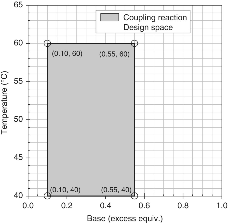
FIGURE 50.34 Expanded design space using variable reaction time.
Source: From Ref. [34]. Reprinted with Permission. Copyright (2016) American Chemical Society.
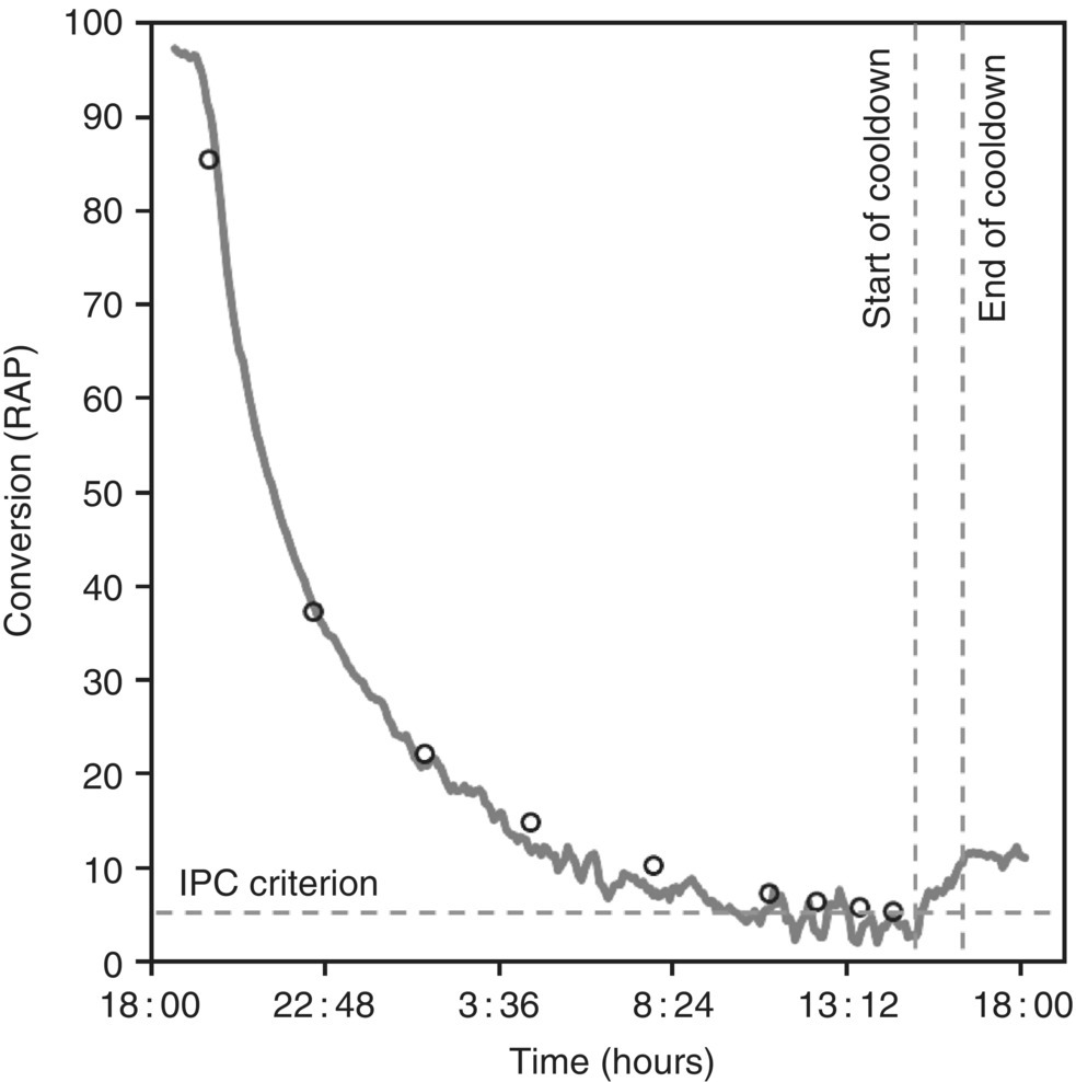
FIGURE 50.35 Reaction monitoring using Raman (–) and HPLC (○).
TABLE 50.18 Elements of Control Strategy for a Final Intermediate
| Final Intermediate Specifications | Type of Control | ||
| Procedural Controls | Material Attributes | Parameter Controls | |
| Impurity A, NMT 0.3% Impurity B, NMT 0.2% Input 2, NMT 0.3% |
Crystallization of Final Intermediate and drug substance shown to purge Impurities A and B, respectively | Attribute specification control on input materials: assay; impurity specifications; water content and alcohol content In‐process controls: testing for Input 2 and impurities in workup |
Design space controls Impurities within limits Operational controls for residual water, alcohol, and oxygen in nitrogen Parameter control during crystallization and drying |
50.7 CONCLUSIONS
The case studies shown in this chapter highlight how impurity formation in reaction steps is often influenced by a combination of process parameters and MAs. The complexity of these scenarios makes the adoption of multivariate approaches indispensable to define a dependable functional relationship between process parameters and QAs. While there will continue to be rapid advances in tools and methodologies to simplify the collection and analysis of data, some of the core principles outlined in the chapter will remain relevant for the foreseeable future. The value proposition of an enhanced strategy that presents the design space in a regulatory submission continues to evolve with different cost–benefit perspectives. However, the importance of this approach to generate critical knowledge toward the design and development of robust processes that reliably assure product quality is indisputable. This should be the ultimate benefit that motivates this paradigm of process development.
50.8 GLOSSARY OF TERMS
- API
- Active pharmaceutical ingredient. Substance or mixture of substances that constitute the active ingredient of the drug product.
- ATR
- Attenuated total reflection. Sampling technique used in spectroscopic analysis that facilitates the direct study of solid, liquid, or gases with little or no sample preparation.
- Center point
- An experiment with all numerical factor levels set at their midpoint value.
- Central composite design
- A design for response surface methods that is composed of a core two‐level factorial plus axial points and center points.
- Contour plot
- Topographical map drawn from a mathematical model, usually in conjunction with response surface methods for experimental design. Each contour represents a continuous response at a fixed value.
- DOE
- Design of experiment. Methodical approach to determine and understand how the parameters of a process affect the performance of that process.
- ICH
- International Council for Harmonization of Technical Requirements for Pharmaceuticals for Human Use. ICH's mission is to achieve greater harmonization worldwide to ensure that safe, effective, and high quality medicines are developed and registered in the most resource‐efficient manner.
- ICP‐MS
- Inductively coupled plasma mass spectrometry.
- IR
- Infrared spectroscopy.
- GC
- Gas chromatography. Chromatographic technique in which the mobile phase is a gas used to separate compounds that can be vaporized.
- GTIs
- Genotoxic impurities. Compounds that have been demonstrated to induce genetic mutations and have the potential to cause cancer in humans.
- KF
- Karl Fischer titration. Volumetric or coulometric method for the determination of moisture content in a sample.
- kL a
- Volumetric mass transfer coefficient. Experimental measure in reciprocal time that represents the rate of mass transfer in a given reactor and mode of operation.
- LC‐MS
- Liquid chromatography–mass spectrometry. Analytical technique that combines liquid chromatography with mass spectrometry.
- LLS
- Laser light scattering. Laser diffraction technique used to analyze particle size distribution in the nm‐to‐mm range.
- NMT
- No more than.
- p‐TsOEt
- Ethyl p‐toluenesulfonate. Alkylating agent and potentially genotoxic impurity that requires a control strategy in process development.
- PAT
- Process analytical technologies. Tools for designing, analyzing, and controlling manufacturing through timely measurements of critical quality and performance attributes of raw and in‐process materials. See Chapter 42.
- PXRD
- Powder X‐ray diffraction. Analytical technique primarily used for phase identification of a crystalline material. The analyzed material is finely ground and homogenized, and average bulk composition is determined.
- QbD
- Quality by design. A systematic approach to development that begins with predefined objectives and emphasizes product and process understanding and process control, based on sound science and quality risk management.
- RAP
- Relative area percent. Estimation of percent composition that divides the area of each peak by the total area of all peaks and multiplies by 100%. Assumes that all the mixture components cause the same response in the detector.
- RMSE
- Root mean square error. The square root of the residual mean squared error. It estimates the standard deviation associated with experimental error.
- TTC
- Threshold of Toxicological Concern for genotoxic impurities. Refers to a threshold exposure level to compounds that does not pose a significant risk for carcinogenicity or other toxic effects.
REFERENCES
- 1. ICH Q11 (2011). Development and Manufacture of Drug Substances (Chemical Entities and Biotechnological/Biological Entities). Rockville, MD: U.S. Department of Health and Human Services, Food and Drug Administration, Center for Drug Evaluation and Research (CDER).
- 2. ICH (2009). Harmonised tripartite guideline: pharmaceutical development Q8 (R2). International Conference on Harmonisation of Technical Requirements for Registration of Pharmaceuticals for Human Use, Geneva (August 2009).
- 3. Yu, L.X., Lionberger, R., Olson, M.C. et al. (2009). Pharmaceutical Technology 33 (10): 122–127.
- 4. Lee, H. (ed.) (2014). Pharmaceutical Industry Practices on Genotoxic Impurities. Boca Raton, FL: CRC Press, Taylor & Francis.
- 5. Sakuramill Sakuramil S2 mock of ICH Q11 Guideline regarding development and manufacture of drug substance. http://www.nihs.go.jp/drug/section3/H23SakuramillMock(Eng).pdf (accessed 13 November 2018).
- 6. ICH (2009). ICH Harmonised Tripartite Guideline: Q8 (R2) Pharmaceutical Development. https://www.ich.org/fileadmin/Public_Web_Site/ICH_Products/Guidelines/Quality/Q8_R1/Step4/Q8_R2_Guideline.pdf (accessed 13 November 2018).
- 7. Thomson, N.M., Singer, R., Seibert, K.D. et al. (2015). Organic Process Research and Development 19: 935–948.
- 8. Glodek, M., Liebowitz, S., McCarthy, R. et al. (2006). Pharmaceutical Engineering 26: 1–11.
- 9. Weissman, S.A. and Anderson, N.G. (2015). Organic Process Research and Development 19: 1605–1633.
- 10. Domagalski, N.R., Mack, B.C., and Tabora, J.E. (2015). Organic Process Research and Development 19: 1667–1682.
- 11. Bakeev, K.A. (2010). Process Analytical Technology: Spectroscopic Tools and Implementation Strategies for the Chemical and Pharmaceutical Industries, 2e. Chichester: Wiley.
- 12. Zaborenko, N., Linder, R.J., Braden, T.M. et al. (2015). Organic Process Research and Development 19: 1231–1243.
- 13. Helfferich, F. (2004). Kinetics of Multistep Reactions, 2e, 7–16. Amsterdam: Elsevier.
- 14. Hannon, J. (2011). Characterization and first principles prediction of API reaction systems. In: Chemical Engineering in the Pharmaceutical Industry. R&D to Manufacturing (ed. D.J. am Ende). Hoboken: Wiley.
- 15. Boudart, M. (1991). Kinetics of Chemical Processes. London: Butterworth‐Heinemann, Reed Publishing.
- 16. Murzin, D.Y. and Salmi, T. (2016). Catalytic Kinetics: Chemistry and Engineering, 2e. Cambridge: Elsevier.
- 17. Cussler, E.L. (1997). Diffusion: Mass Transfer in Fluid Systems, 2e. London: Cambridge University Press.
- 18. (a) Carpenter, B.K. (1984). Determination of Organic Reaction Mechanisms. New York: Wiley. (b) Espenson, J.H. (1995). Chemical Kinetics and Reaction Mechanisms, 2e. New York: McGraw‐Hill. (c) Houston, P.L. (2006). Chemical Kinetics and Reaction Dynamics. New York: Dover Publications, Inc.
- 19. Caron, S. and Thomson, N.M. (2015). The Journal of Organic Chemistry 80: 2943–2958.
- 20. Madelaine, G., Lhoussaine, C., and Niehren, J. (2015). Structural simplification of chemical reaction networks preserving deterministic semantics. In: Computational Methods in Systems Biology. CMSB 2015, Lecture Notes in Computer Science, vol. 9308 (ed. O. Roux and J. Bourdon). Cham: Springer.
- 21. Klamt, S. and Stelling, J. (2006). Stoichiometric and constraint‐based modeling. In: Systems Modeling in Cellular Biology (ed. Z. Szallasi, J. Stelling and V. Periwal). Cambridge, MA: MIT Press.
- 22. Turányi, T. and Tomlin, A.S. (2014). Analysis of Kinetic Reaction Mechanisms. Berlin, Heidelberg: Springer−Verlag.
- 23. Burt, J.L., Braem, A.D., Ramirez, A. et al. (2011). The International Journal of Pharmaceutics 6: 181–192.
- 24. Thomas, B.G. and Brimacombe, J.K. (1997). Process modeling. In: Advanced Physical Chemistry for Process Metallurgy (ed. N. Sano, W.‐K. Lu, P.V. Riboud and M. Maeda). San Diego, CA: Academic Press.
- 25. Ekins, S. (2006). Computer Applications in Pharmaceutical Research and Development, 2e. Hoboken, NJ: Wiley.
- 26. Montgomery, D.C. (2013). Design and Analysis of Experiments, 8e. Danvers, MA: Wiley.
- 27. Oehlert, G.W. (2000). A First Course in Design and Analysis of Experiments. New York: W. H. Freeman.
- 28. Robinson, T.J. (2014). Box‐Behnken Designs. Wiley Stats Ref: Statistics Reference Online.
- 29. (a) Dean, A.M. and Voss, D. (1999). Design and Analysis of Experiments. New York: Springer‐Verlag. (b) Klimberg, R. and McCullough, B.D. (2016). Fundamentals of Predictive Analytics with JMP®, 2e. Cary, NC: SAS Institute.
- 30. U.S. Food and Drug Administration (2012). Guidance for Industry Q8, Q9, & Q10 Questions and Answers – Appendix Q&As from Training Sessions. U.S. Department of Health and Human Services Food and Drug Administration Center for Drug Evaluation and Research (CDER) Center for Biologics Evaluation and Research (CBER) July 2012 ICH.
- 31. European Medicines Agency (2013). Questions and Answers on Design Space Verification. Retrieved 2 May 2017. https://www.ema.europa.eu/documents/other/questions‐answers‐design‐space‐verification_en.pdf (accessed 13 November 2018).
- 32. Garcia, T., McCurdy, V., Watson, T.N. et al. (2012). The Journal of Pharmaceutical Innovation 7: 13–18.
- 33. Watson, T.J., Bonsignore, H., Callaghan‐Manning, E.A. et al. (2013). The Journal of Pharmaceutical Innovation 8: 67–71.
- 34. Hallow, D.M., Mudryk, B.M., Braem, A.D. et al. (2010). The Journal of Pharmaceutical Innovation 5: 193–203.
- 35. ICH (2011). ICH quality implementation working group points to (R2) ICH−Endorsed Guide for ICH Q8/Q9/Q10 Implementation. Document date: 6 December 2011.
- 36. Ramirez, A., Hallow, D.M., Fenster, M.D.B. et al. (2016). Organic Process Research and Development 20: 1781–1791.
- 37. Tom, N.J., Simon, W.M., Frost, H.N., and Ewing, M. (2004). Tetrahedron Letters 45: 905–906.
- 38. (a) Prausnitz, J.M., Lichtenthaler, R.N., and Azevedo, E.G. (1986). Molecular Thermodynamics of Fluid‐Phase Equilibria. Englewood Cliffs, NJ: Prentice Hall. (b) Grant, D.J.W., Mehdizadeh, M., Chow, A.H.L., and Fairbrother, J.E. (1984). The International Journal of Pharmaceutics 18: 25–38.
