
16
DESIGN AND SELECTION OF CONTINUOUS REACTORS FOR PHARMACEUTICAL MANUFACTURING
Martin D. Johnson, Scott A. May, Michael E. Kopach, Jennifer McClary Groh, Timothy Braden, Vaidyaraman Shankarraman, and Jeremy Miles Merritt
Eli Lilly and Company, Indianapolis, IN, USA
16.1 DRIVERS FOR CONTINUOUS REACTIONS IN DRUG SUBSTANCE MANUFACTURING
Continuous processing applications in the pharmaceutical industry have been increasing in recent years [1]. There are many reasons why an API manufacturer may choose to run chemical reactions in continuous mode instead of batch. Typical drivers for choosing continuous instead of batch reaction are fast kinetics, highly exothermic heats of reaction, hazardous reagents, extreme temperatures and pressures, and high throughput. Yield and selectivity may be better for fast reactions in series with unstable intermediates [2]. Safety may be improved for highly exothermic reactions [3]. Operating ranges may be wider, and safety may be improved for high pressure reactions with hazardous gas reagents such as hydrogenations, hydroformylations, aerobic oxidations, and carbonylations. Operating ranges may be larger, and safety may be improved for reactions at extreme temperatures less than −40 °C or greater than 200 °C or superheated reactions with vapor pressure greater than 50 bar at reaction temperature [4]. There are safety advantages of minimizing volumes and maximizing heat transfer rates for reactions with hazardous reagents, potential for thermal runaway or large exotherms [5]. Safety is improved for reactions with hazardous reagents like reactions with hydrazine, bromonitromethane, diazomethane [6], sodium cyanide, methanesulfonyl cyanide, and cyanogen chloride [7]. If there is an advantage to running with no headspace, such as organic azide or tetrazole formations where hydrazoic acid would partition into the headspace of the batch reactor, then a plug flow reactors (PFR) may be superior to batch because it operates 100% liquid filled [8]. If the impurity profile is improved by all‐at‐once addition, coaddition, fast heat‐up, and/or fast cooldown, then a PFR or a continuous stirred tank reactor (CSTR) may be superior to batch. This depends on the kinetics of the side reactions relative to the main desired reaction. Continuous can provide throughput advantages and debottlenecking for high volume products [9]. End‐to‐end fully continuous processes offer advantages of quality control, extreme operating conditions, telescoping, and introducing excipients further upstream to improve processing API to drug product [10]. The use of continuous reactors in the pharmaceutical industry is rapidly increasing [11]. Product consistency advantages can be achieved via continuous processing because of steady‐state operation, feedback control, and real‐time product quality information by online process analytical technology (PAT). It aligns with quality by design (QbD) principles, and implementation of continuous processes is encouraged and supported by the FDA [12].
There are several additional criteria to look for in the batch reaction that may cause one to think about continuous. Is the yield or impurity profile sensitive to reaction time? Are there significant late‐forming impurities? Is the product unstable to end‐of‐reaction conditions? If the answer is yes to any of these questions, then consider reaction in a plug flow tube reactor (PFR), because reaction time is more scalable, the late‐forming impurities can be avoided by precise control of time in the reactor, and the unstable product can be quenched in‐line immediately after the precisely controlled reaction time. Is the yield or impurity profile sensitive to mixing rate, heat‐up rate, or cooldown rate? Reagent addition time is more scalable in flow than in batch because of in‐line mixing and because the production‐scale reactors are not as large as batch. Heat‐up and cooldown rates are more scalable in continuous than batch. This is because process liquids flow through heat exchangers at the reactor inlet and outlet. Does the yield or impurity profile benefit from all‐at‐once mixing of reagents? If so, then a PFR is a better reactor choice than batch for all‐at‐once stoichiometric reagent mixing because of the ability to control (or remove) heat from an exothermic reaction. Is there a lag time or delayed catalyst initiation time in the batch reactor? In this case, the advantage of a CSTR is that the reaction is always operating at the end‐of‐reaction conditions. Is the product cytotoxic or highly potent? Using continuous processing, cytotoxic API production may be achieved in inexpensive, dedicated, and “disposable” equipment sets for production of low volume (<1000 kg/year) cytotoxic APIs in laboratory fume hoods [13]. Is it difficult to recover a batch in the event of operational problems? For example, if the catalyst deactivates because of something like poor inertion and if it is difficult to recover from this event by simply adding more catalyst, then the flow advantage of the PFR is that there is less material at risk due to the small reactor volume compared with the total production volume (one to one in batch operations).
16.2 TWO MAIN CATEGORIES OF CONTINUOUS REACTORS: PFRs AND CSTRs
Continuous reactors fall into two main categories, CSTR and plug flow with dispersion reactor (PFDR) [14]. They are shown schematically in Figure 16.1.

FIGURE 16.1 Schematic drawings of CSTR and PFDR. CA0 is initial concentration of reagent A entering the reactor, CA is concentration of reagent A in PFR, and CAF is final concentration of reagent A exiting the reactors, which is the same as the concentration of reagent A everywhere in the ideal CSTR.
The design equations are derived by solving the material balance for conversion versus mean residence time (τ) or distance after making simplifying assumptions [15]. The design equations relate changes in concentration with time to flow of reacting species in and out of reactor and species formation/disappearance by chemical reaction. The design equation for the CSTR assumes no spatial changes within the reactor and no change with time at steady state. If the mixing time is sufficiently fast compared with the mean residence time, then the entire contents of the reactor remain at outlet concentrations. The simplified design equation for the PFDR assumes no change with time for a given location in the reactor, but change in conversion with distance along the axial direction from reactor inlet to outlet. The PFDRs are commonly called PFRs, but PFR implies perfect mixing in the radial direction and no mixing in the axial direction, which is not true for real reactors. All real reactors have some degree of axial dispersion, especially with laminar flow homogeneous liquids. If the axial dispersion number is small enough so that it has negligible impact on conversion versus τ, then the PFDRs are called PFRs. This chapter contains an example of quantifying axial dispersion and then modeling whether or not it has significant impact on conversion versus time in real rectors. There are many types of PFRs such as:
- Microreactors.
- Static mix tube reactors.
- Open tube or pipe reactors.
- Oscillatory baffled tube reactors.
- Flow tube or structured channel reactors that have alternative energy input like microwave, photo, electro, or sono energy input.
With proper engineering design, each of these variations can be designed to minimize axial dispersion such that highly plug flow profiles result.
Reaction conversion versus τ is different in a CSTR than in a PFR, and the respective residence time distributions (RTD) are also very different. Much longer residence times are required for full conversion in a CSTR compared with a PFR, unless the reaction rate is zero order. Example calculations are shown in this chapter to illustrate this point.
Judging by the number of published examples and the number of commercially available continuous reactor systems, PFRs are more commonly applied than CSTRs. PFRs maximize heat transfer A/V compared with stirred tanks, especially if they are microreactors, i.e. characteristic dimension less than 1 mm. A PFR minimizes total reactor volume and thus τ in the reactor for a given conversion. A PFR minimizes transition time and volume to reach a new steady state after a step change in process parameter because of narrow RTD. The PFR can run 100% liquid filled and as a consequence is the best reactor choice to eliminate headspace. This also helps to minimize equivalents of gas reagent for two‐phase vapor–liquid reactions. The working volume of research‐scale PFRs can be less than 0.1 ml; therefore they minimize materials required for research and development. Compared with CSTRs in series or intermittent flow CSTRs, the PFRs can be lower in complexity and lower in cost. One of the biggest challenges is to maintain solubility of reagents and reaction products in PFRs. Most PFRs are not capable of solids in flow because of fouling or blockage. Solids in packed columns are acceptable, for example, packed catalyst bed reactors, but the particle size of the solids should be greater than 100 μm to minimize pressure drop across the bed.
On the other hand, CSTRs, CSTRs in series, or intermittent flow CSTRs may be selected instead of PFRs in certain circumstances. These reactors are more suitable for heterogeneous systems, including slurry flow such as reactive crystallizations, reaction with solid precipitate, or reaction with solid reagent feeds like Grignard formation reactions with solid magnesium reagent. CSTRs tolerate and buffer out fluctuations and/or pulsing of reagent feeds. In fact, a useful reactor configuration is a small CSTR followed by a PFR, where the CSTR dampens out fluctuations in stoichiometry of two reagents combining prior to entering the PFR. While PFRs need precise flow control especially for multiple reagents, CSTRs are more forgiving of short oscillations in flow control. If stoichiometry is critical and the pump flow rates oscillate, then consider CSTRs. CSTRs can be stopped and restarted without loss of mixing during flow stoppage. Also, mixing is independent of flow rate in CSTRs. CSTRs achieve fast liquid–liquid two‐phase mixing over a wider range of scales and reaction times, for example, a one hour reaction time in production‐scale reactor. CSTRs help to overcome induction time or lag time in reaction kinetics, e.g. autocatalytic reaction, because they operate at “end‐of‐reaction” conditions at steady state. Also, because CSTRs do not run completely liquid filled, it is more feasible to adjust residence time in the reactor without changing liquid flow rate.
Furthermore, the choice of PFR versus CSTR versus batch depends on the best method of reagent addition. Reaction kinetics will determine the best reactor configuration for maximizing yield and minimizing side reactions and impurities. In any of the reactor configurations (batch, plug flow, continuous CSTRs, or intermittent flow CSTR), one can easily use kinetics from the batch reactions to design and size the continuous reactor for full conversion. The bigger challenge is understanding and predicting the impurity profile for the different reactor configurations. For a reaction A + B → C, if the impurity profile and yield are most favorable when reagent B is added in a slow and controlled manner to a vessel containing reagent A, then batch and intermittent flow CSTR are better reactor choices than a PFR or true CSTR. A PFR with multiple addition points of reagent B along the length of the reactor is an alternative, but it requires more pumps and mass flow controllers. A mathematical example is given in Section 16.5. If impurity profile and yield are best for an all‐at‐once addition, then a PFR is the best choice. Batch is usually not practical for all‐at‐once stoichiometric addition because of safety concerns and heat transfer limitations. If yield and selectivity are most favorable as a result of slow coaddition of both A and B at stoichiometric ratios (i.e. coaddition) while keeping the conversion high in the reactor at all times, then a CSTR is the best reactor choice.
16.3 EXAMPLE OF COILED TUBE PFR FOR TWO‐PHASE GAS–LIQUID REACTIONS
An asymmetric hydrogenation reaction operating at 68 bar hydrogen produced 144 kg of penultimate using a 73 L coiled tube PFR [16]. The reactor and the downstream separations and purification unit operations were run in laboratory facilities at 13 kg/day throughput. The hydrogenation was in a special laboratory facility with all explosion proof equipment, utilities, and lighting, high air volume turnovers, specialized doors, and blowout walls. The reaction scheme is shown below in Scheme 16.1. It was a challenging hydrogenation of a tetrasubstituted enone.

SCHEME 16.1 Rhodium‐catalyzed asymmetric hydrogenation.
The rhodium and Josiphos homogeneous catalyst ligand system was very oxygen sensitive. Running the reaction continuous rather than batch provided advantages for excluding oxygen, because the reactor only needed to be inerted once at the beginning of the campaign. The catalyst system was also very expensive. To be economically viable, this reaction required a 2000 : 1 substrate to catalyst ratio (S : C) and high pressure hydrogen (68 bar) to maintain a high dissolved H2 concentration. The enone substrate was 0.15 M in 2.5 : 1 ethyl acetate/methanol, and the dissolved H2 concentration was expected to be on the same order or magnitude at the elevated pressure. Batch processing is normally the default option, but a 68 bar rated autoclave was not available at the selected manufacturing facility for this product. A capital spend was needed to support either a batch or continuous process.
There are several good references for determining kinetics in continuous reactors [17]. Reaction kinetics were measured in a well‐mixed batch PARR autoclave at research scale. Conversion versus time was measured in the autoclave, and the results are listed in Table 16.1.
TABLE 16.1 Hydrogenation Reaction Experimental Rate Data
| Time (h) | Conversion (%) |
| 2.0 | 69.7 |
| 3.0 | 83.1 |
| 4.0 | 92.3 |
| 5.6 | 96.9 |
| 6.8 | 98.5 |
| 8.4 | 99.5 |
Temperature 70 °C and pressure 68 bar.
Plotting the natural log of C/Co versus time gives a straight line with slope equal to the reaction rate constant for a first‐order reaction, where C is concentration of starting reagent at time t and Co is initial concentration.
The rate expression is
where
- k is the first‐order rate constant.
By separating variables and integrating, this becomes


A plot of the natural log of C/Co versus time is shown in Figure 16.2.
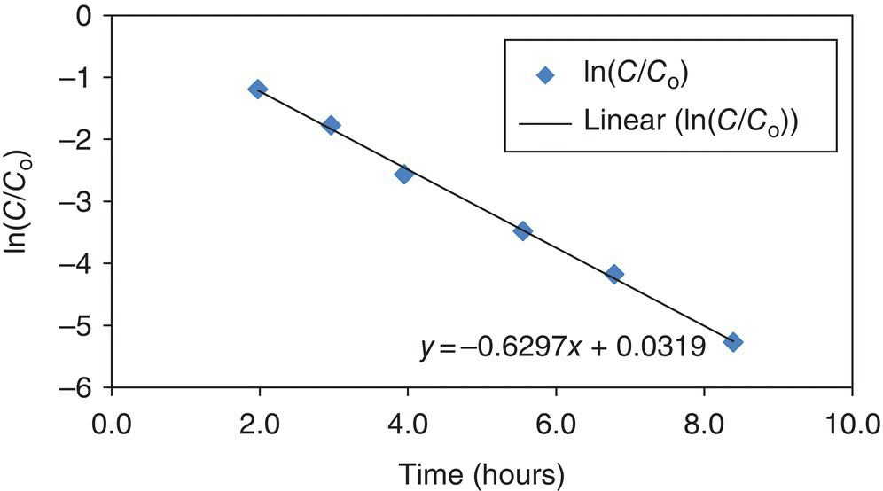
FIGURE 16.2 Plot of the natural log of C/Co versus time to confirm first‐order reaction and determine rate constant.
In this example, the product concentration is log linear; therefore the reaction is first order or pseudo first order with k = 0.63/h within the time period investigated. The first‐order reaction rate model with k = 0.63/h is plotted with the actual conversion versus time data in Figure 16.3 and Table 16.1.
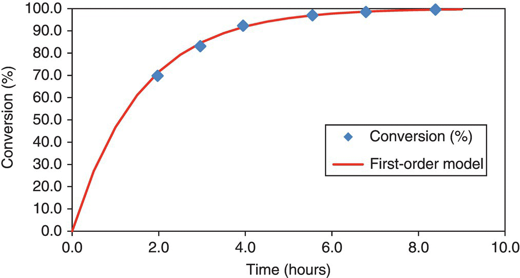
FIGURE 16.3 Conversion versus time and first‐order reaction rate model fit to the data for asymmetric hydrogenation. Reaction at 70 °C and 68 bar.
Overall gas–liquid mass transfer coefficient, kLa, was the order of 0.01–0.1/s; therefore conversion versus time was likely not mass transfer rate limited. The kinetic data informs the choice of reactor type: batch versus PFR versus CSTR. The rate data was used to predict how long the reaction must run to reach a desired 99.9% conversion level in batch mode and what is the required reaction time to reach the same conversion in the PFR or CSTR.
In the PFR, the reagent solution, catalyst solution, and reagent gas flowed cocurrently through the coiled tubes. A simplified schematic of the reactor system is shown in Figure 16.6.

FIGURE 16.6 Schematic of PFR for two‐phase reaction with hydrogen gas.
Photographs of the 73 L reactor are shown in Figure 16.7. The overall height and diameter of the cylindrical coiled tubing assembly was designed to fit inside an existing 0.91 m diameter jacketed single plate filter that was used as a constant temperature bath, also shown in Figure 16.7.
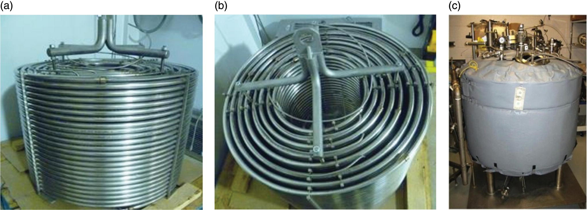
FIGURE 16.7 Pictures of (a) 73 L coiled tube PFR side view, (b) top view, and (c) constant temperature heating bath for submerging the reactor.
The PFR was constructed of 316 L stainless steel tubing with outer diameter (o.d.) = 19.1 mm, inner diameter (i.d.) = 16.5 mm, and L = 340 m. Overall L/d was about 20 600, which is unusually large for tubular reactor designs. This is because the reactor was designed for 12 hours τ and flow was in the laminar regime. Reynolds number was about 250 in the flow tube reactor. In the laminar regime, the larger the L/d, the lower the overall reactor axial dispersion number [18]. Due to the low linear velocity because of the 12 hours τ, the reactor operated with pressure drop of only about 10 psi; thus the pressure drop was not problematic. Reactor cost and ease of fabrication were the practical limitations on higher L/d in this case. The tubing was formed into eight concentric cylindrical coils 0.53 m tall and ranging from 0.36 to 0.80 m diameter as pictured in Figure 16.7. Vapor and liquid flowed cocurrently through each of the eight coils in series in the uphill direction starting with the outside coil. These individual coils were linked by down‐jumper tubes constructed from 316 L stainless steel tubing with o.d. = 6.35 mm and i.d. = 4.57 mm. The reactor was designed with these narrow diameter down‐jumpers to maintain greater than 99% of the total reactor volume in the uphill flow direction, which helped the reactor run more liquid filled in the forward direction. This also made it possible to almost completely empty the reactor by pushing with nitrogen in the reverse direction at the end of the production. There was no mechanical mixing of the hydrogen and liquid throughout the length of the tube. Gas–liquid mixing was sufficient so that conversion versus time was the same as in a well‐mixed batch reactor.
The reactor was designed to be low cost so that it was dedicated to this specific chemistry and this rhodium catalyst and then disposed when no longer needed for the product. This reduced the cleaning burden, eliminated the possibility of cross‐contamination, and eliminated other metal catalyst from the possibility of catalyzing undesired side reactions. The 73 L coiled tube PFR in this example cost $16 000.
Using the PFDR model, vessel dispersion number D/uL can be calculated by fitting experimental F‐curve data to the basic differential equation representing dispersion by numerically solving for D/uL and θ as shown in the following equation:

- D = Taylor longitudinal dispersion coefficient that incorporates the effect of both diffusion and convection
- u = average flow velocity
- L = vessel length
- C = concentration
- θ = dimensionless time (t/τ), where τ is mean residence time
- Z = dimensionless length (x/L)
From θ and the recorded time for each data point, we can calculate τ. The C‐curve characterizes spreading of a pulse tracer injection into the inlet of a flow tube reactor as it travels along the length of the reactor, also known as residence time distribution. See chemical engineering textbooks for details on the methods and analyses [15]. For small extents of dispersion, D/uL < 0.01, the basic differential equation representing dispersion can be solved analytically to give the following symmetrical C‐curve:

Given that the F‐curve is the integral of the C‐curve, this equation was used to quantify D/uL and θ for the experimental F‐curve using a simple Excel® spreadsheet.
Figure 16.8 shows the experimental F‐curve data collected during startup transition of the 73 L coiled tube reactor. The reactor initially started filled with solvent. At time zero, the reagent solution with enone, the dissolved catalyst + ligand solution, and hydrogen gas started flowing into the reactor. The figure plots product concentration at the reactor exit versus normalized time, t/τ. t/τ = 1 corresponds to 11.8 hours.
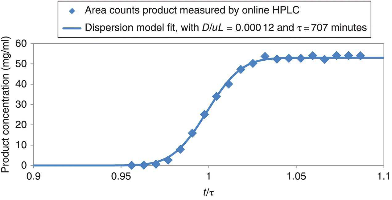
FIGURE 16.8 Experimental F‐curve data and model fit for startup transition of a 73 L continuous hydrogenation reactor.
In this example, the axial dispersion number, D/uL, was 0.000 12, and τ was 11.8 hours (Figure 16.8). Thus, the continuous reactor exhibited nearly ideal plug flow characteristics. This is a remarkably low axial dispersion number given that the reactor is in the laminar regime. Reynolds number in the reactor was only about 250 (liquid density 0.9 g/ml, internal diameter 16 mm, linear velocity 8 mm/s, viscosity about 0.45 cp). The gas + liquid two‐phase flow decreases axial dispersion compared with liquid‐only flow because the gas bubbles disrupt the parabolic velocity profile and cause some mixing in the radial direction [16]. Even without the gas, however, axial dispersion would be low in this reactor at Reynolds number about 250 because of the extremely high length to diameter ratio, as explained elsewhere [16]. Steady state was achieved in this example after about 1.03 × τ during startup transition from a solvent‐filled reactor, as shown in Figure 16.8. Target reaction τ was 12 hours, but actual was 11.8 hours. This emphasizes the value of measuring and modeling the startup transition curve, because it quantifies the actual τ. In addition to many other things, τ depends on % vapor space in the reactor, which is difficult to predict because it depends on relative gas versus liquid linear velocities. This makes it difficult to know actual τ without measuring the startup transition curve. A nonreactive tracer could also be used, but this was a production run for a pharmaceutical intermediate, so any extra additives are scrutinized.
Numerical modeling of the one‐dimensional convective diffusion equation was performed to illustrate the effects of dispersion in the 73 L PFR. The partial differential equation was solved using gPROMS custom modeler [19] discretizating along the length of the tube reactor. Backward finite differences were used, and a Danckwerts boundary condition was employed [20]. Numerical diffusion dictated the number of discretization points needed in order to simulate very low D/uL scenarios. Approximately 10 000 discretization grid points were needed to ensure numerical diffusion was small relative to the diffusion expected for a D/uL of 1.2e‐4. Analytical expressions were used for the simulation of ideal PFR and CSTR cases.
First the effect of dispersion on the steady‐state conversion at the exit of the tube reactor was examined. The numerical results of the model are shown in Figure 16.9. The limiting conversion at low D/uL is due to the residence time needed to achieve the design criteria of 99.9% conversion. At high D/uL the limiting case for an ideal CSTR is obtained. The conversion is insensitive to dispersion for D/uL < 1e‐3.

FIGURE 16.9 Steady‐state conversion at the outlet of the PFR as a function of the dispersion coefficient.
Next the steady‐state fractional conversion was simulated as a function of distance along the PFR for several representative values of D/uL, and the results are shown in Figure 16.10. At a D/uL of 1e‐4, the concentration profile is virtually indistinguishable from the ideal PFR curve. For an ideal CSTR (infinitely high D/uL), the concentration at L = 0 drops (instantaneously) to the steady‐state conversion of a CSTR with 11.8 hours τ.
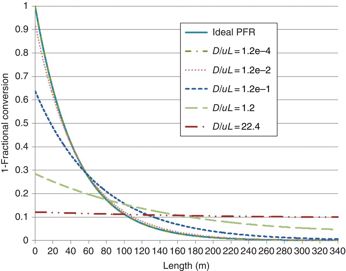
FIGURE 16.10 Steady‐state reaction conversion as a function of distance in the PFR for representative values of D/uL.
Figure 16.11 shows the comparison of ideal PFR and the real PFR with D/uL = 0.000 12 for the last 10 m of the reactor. The difference in conversion versus distance along the reactor is quantifiable but negligible for this low value of axial dispersion. The ideal PFR curve was done analytically, and the plug flow with dispersion curve was done using the gPROMS numerical solver and 10 000 grid points. The simulations show that conversion versus distance is slightly less for the reactor with dispersion but clearly negligible for practical purposes.

FIGURE 16.11 Steady‐state reaction fractional conversion as a function of distance in the PFR for the final 10 m and comparison to ideal plug flow.
To illustrate the effect of dispersion when not at steady state, concentration profiles along the length of the PFR are shown in Figure 16.12 for time = 1 hour after switch to the reactive feeds. For an ideal PFR the step change is infinitely narrow; however for larger values of dispersion, the step change gradually broadens out.
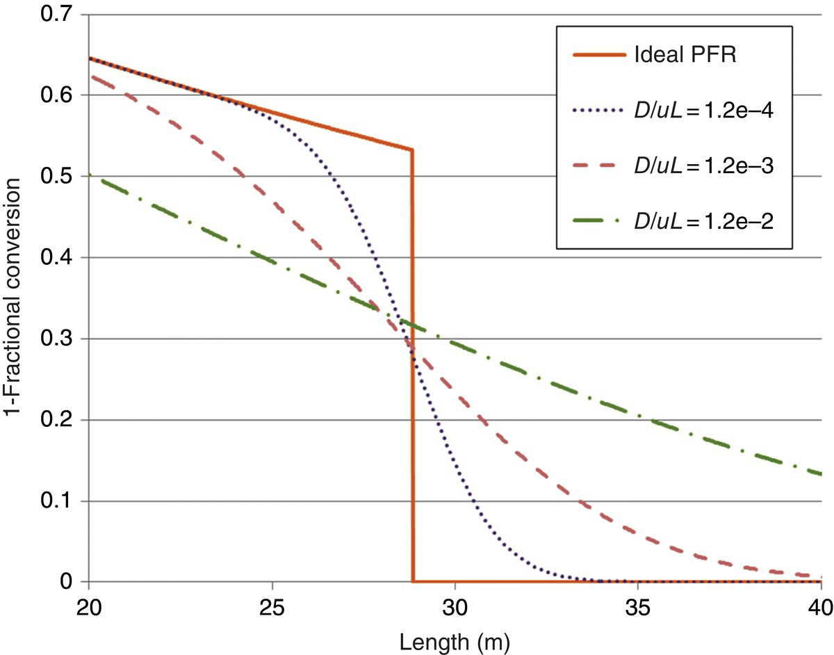
FIGURE 16.12 Reaction conversion as a function of distance in the PFR for different values of D/uL and time = 1 hour after switchover of the feeds from solvent to reagents in the startup transition.
16.4 EXAMPLE OF CSTR FOR GRIGNARD FORMATION REACTION WITH SEQUESTERED Mg SOLIDS
A continuous Grignard formation reaction was run in a CSTR with sequestered magnesium solids for reasons of safety and minimizing key impurities. The reaction is shown below in the Scheme 16.2.
SCHEME 16.2 Grignard reaction in a CSTR.
The key impurities are shown below.

The Wurtz coupling impurity was minimized by maintaining a high stoichiometric ratio of magnesium to aryl bromide starting material, the proteo impurity was reduced by minimizing water, and phenol was decreased by minimizing oxygen. Control of each of these impurities was easier to accomplish in a continuous reactor compared with batch. Oxygen and water are easier to minimize in a continuous reactor versus batch because the reactor is inerted and dried once and then remains inert and dry at steady state. The explanation for why the CSTR maintained high stoichiometric ratio of magnesium to aryl bromide starting material is given in the following discussion.
Liquid solutions were continuously pumped into the reactor containing a large molar excess of a solid activated magnesium metal, while liquid product solution was continuously pumped out, with the solid magnesium being sequestered in the reactor. Solid magnesium particles were periodically added once every four hours at an average rate equal to the molar feed rate of the starting material. In other words, Mg solids were added at a rate to match consumption. The magnesium was added in a very simple way. In a 6 L pilot‐scale reactor, a 2 in diameter cap was removed from a nozzle on the top of a glass reactor, and the Mg was poured into the vessel from a beaker through a funnel. In a 100 L manufacturing reactor, the port on the Hastelloy reactor was removed, and Mg was poured into the vessel from 1 gal wide‐mouth containers inside a glove bag. The freshly added metal rapidly activated when it mixed with the existing Grignard solution without the need for any additional activating agent. The kinetics of the Grignard formation reaction were extremely fast, achieving greater than 99% conversion in a single CSTR with a 1 hour mean residence time. This corresponds to a batch reaction with 99% conversion in 26 seconds, as described later in this section. A simplified schematic of the reactor system is shown in Figure 16.13.

FIGURE 16.13 Schematic of CSTR for Grignard formation reaction with sequestered Mg solids.
Keeping solid magnesium particles in the CSTR was a key operational challenge. The two main methods/devices used to prevent magnesium from exiting the system were the settling pipe in the CSTR and the magnesium settling trap immediately downstream from the CSTR. These are described in more detail in the literature [21]. A 6 L pilot‐scale reactor operated at the 4.5 L fill level and a 100 L manufacturing‐scale reactor operated at the 45 L fill level. The 100 L CSTR was used to generate 4000 L of 0.85 M Grignard reagent solution for an API starting material. Forward processing of the Grignard reagent into a coupling reaction and subsequent workup and isolation were done in batch 8000 L vessels. There were significant safety advantages of running the reaction in a 100 L CSTR instead of 8000 L batch reactor. The Grignard formation reaction was highly exothermic, initiation was difficult, and the reaction had runaway potential; therefore minimizing the size of the reactor minimized the safety risks. The Grignard initiation was confirmed in the CSTR by stopping flow of aryl bromide after five minutes and quantifying the exotherm before continuing. The Grignard was first initiated batch but only at 250 ml reactor scale. A 250 ml CSTR produced enough active Grignard reagent to initiate a 6 L CSTR, and the 6 L CSTR produced enough active Grignard reagent to initiate a 100 L CSTR.
The number of molar equivalents of magnesium in the reactor relative to substrate oscillated. The goal was to keep at least 4 M equiv. Mg in the CSTR relative to substrate, which was greater than 99% Grignard reagent rather than aryl bromide at any time. Therefore, the CSTR started with 8 M equiv., and the first Mg recharge was done after four reactor volume turnovers. Plotting the instantaneous molar equivalents of magnesium in the reactor results in a sawtooth plot over the 96 turnover manufacturing campaign (Figure 16.14). Observe that the Grignard reaction maintained high instantaneous magnesium equivalents (4–8) while achieving usage of 1.04 equiv. of magnesium overall for the manufacturing campaign. This can be compared with 1.5 equiv. of magnesium that would have been used in the batch campaign. This is probably the main reason why the CSTR approach gave less Wurtz coupled impurity compared with the batch reaction approach. In addition, a batch reaction with 1.5 M equiv. of Mg would have resulted in more magnesium to quench at the end, compared with the CSTR manufacturing that used 1.04 M equiv. overall. The magnesium quench liberates hydrogen; therefore the continuous process generated less hydrogen than the batch counterpart would have generated, which was a safety advantage of the CSTR approach.
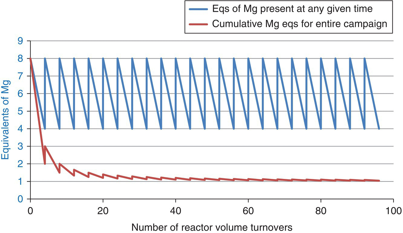
FIGURE 16.14 Instantaneous molar equivalents of magnesium in the reactor and also the overall cumulative molar equivalents of magnesium added for the 96 turnover manufacturing production campaign.
The reaction achieved 99.9% conversion with a 60 minute residence time in a single CSTR operating at 41 °C. Assuming pseudo first‐order reaction process, the rate constant can be calculated:
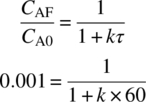
- k = 16/minute
Conversion for different τ can be predicted once the rate constant is known. For example, if the residence time is reduced to 30 minutes, then conversion would drop to 99.8%:
One can calculate what the reaction time would be for 99.9% conversion if the reaction was run isothermally batch. Of course, it is not possible to run this reaction isothermally batch because of the large exotherm and the unrealistically high heat removal rate that would be required:
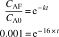
- t = 0.43 minutes
It is important to note that it is not practical to measure this rate constant by running a batch reaction. The adiabatic temperature rise was 130 °C; therefore it would not be possible to keep the reactor temperature at 40 °C during a 26 second reaction. Performing this reaction in batch would also have mass transfer limitations. Therefore running this reaction in a CSTR is a more effective way to experimentally quantify the true kinetics for this fast exothermic reaction.
At pilot scale, the automation system monitored the process with a real‐time energy balance in the 6 L CSTR campaign, in order to prove the reaction was operating at a high conversion. At steady state, the heat removal rate by the cooling jacket was 188 W:

Increasing the incoming feed from room temperature to the reaction temperature consumed 26.4 W:
The steady‐state heat generation rate from reaction was 208 W:


The heat loss to surroundings was assumed zero since the reactor jacket was room temperature.
Real‐time energy balance was 103%, because total heat removed was 214 W and heat generated was 208 W. This real‐time energy balance was an important safety feature of the process, and it was constantly calculated and monitored by the distributed control system (DCS). Automated shutoffs were in place to stop the reagent feeds if the real‐time energy balance was below a limit, preventing the possibility of unreacted aryl bromide reagent accumulating to unsafe levels in the Grignard reactor.
16.5 NUMERICAL MODELING TO SELECT THE BEST REACTOR TYPE FOR MINIMIZING IMPURITIES
A simple hypothetical series–parallel reaction is used next to illustrate that there can be significant differences in impurity profiles for the same reaction depending on the reactor choice (PFR vs. batch with controlled addition vs. CSTR). The reaction and the kinetics (at 25 °C) in this example are
where
- A and B are reactants.
- P is the product.
- Imp is an undesired impurity.
The details of the governing equations and the parameters used in this illustration are listed in Table 16.2. The governing equation for PFR is the same as batch with all‐at‐once addition, because time variable in batch translates to residence time along the reactor for a PFR.
TABLE 16.2 Governing Equations and Parameters Used to Illustrate Difference in Impurity Profile Between PFR, Batch with Controlled Addition (Semi‐batch), and CSTR
| PFR (Batch with All‐at‐Once Addition) | Controlled Addition (Semi‐batch) | Three CSTRs in Series |
cj: Concentration of species j along the reactor (at residence time t) rj: rate of formation per unit volume of species j |
cj: Concentration of species j at time t vf: Ratio of volumetric flow rate of addition stream to volume of reactor rj: Rate of formation per unit volume of species j |
τ: Residence time in each CSTR rj: Rate of formation per unit volume of species j |
| Reaction Rate Expressions |
|
|
| PFR Inlet concentration: Residence time: 1 h |
||
| Controlled Addition (Semi‐batch) Initial concentration in reactor: Addition stream concentration: Addition stream flow rate:4 L/h, initial reactor volume: 3 L, and dosing time: 30 min Reaction time: 1 h |
||
| CSTR: (Three CSTRs in Series with Equal Residence Time) Inlet concentration to CSTR 1: Residence time of each CSTR: 1 h |
||
The concentrations after all reagents are mixed (if there was no reaction) would be the same in all three cases in the table. For the batch with controlled addition over 30 minutes, cA after mixing would be 2 × 3/(3 + 4 × 0.5) = 1.2 M, and cB after mixing would be 4 × 4 × 0.5/(3 + 4 × 0.5) = 1.6 M.
The model for this example was implemented using DynoChem [22]. The governing equations are different between PFR, batch with controlled addition, and CSTRs in series. Even though the kinetics are the same, the impurity profiles are different for the three different reactors. In this example, the PFR with residence time of 1 hour results in 96% in situ yield and 2.5% Imp. Controlled addition of B over 30 minutes, followed by 30 minutes of additional reaction mixing time, results in 94% in situ yield and 1.8% Imp. If this reaction is run using three CSTRs each with 1 hour residence time, an in situ yield of 94% can be achieved, but the impurity level at steady state is 5%. Figure 16.15 shows the impurity level versus conversion of A for (i) a PFR, (ii) batch with controlled addition, and (iii) three equal volume CSTRs in series.
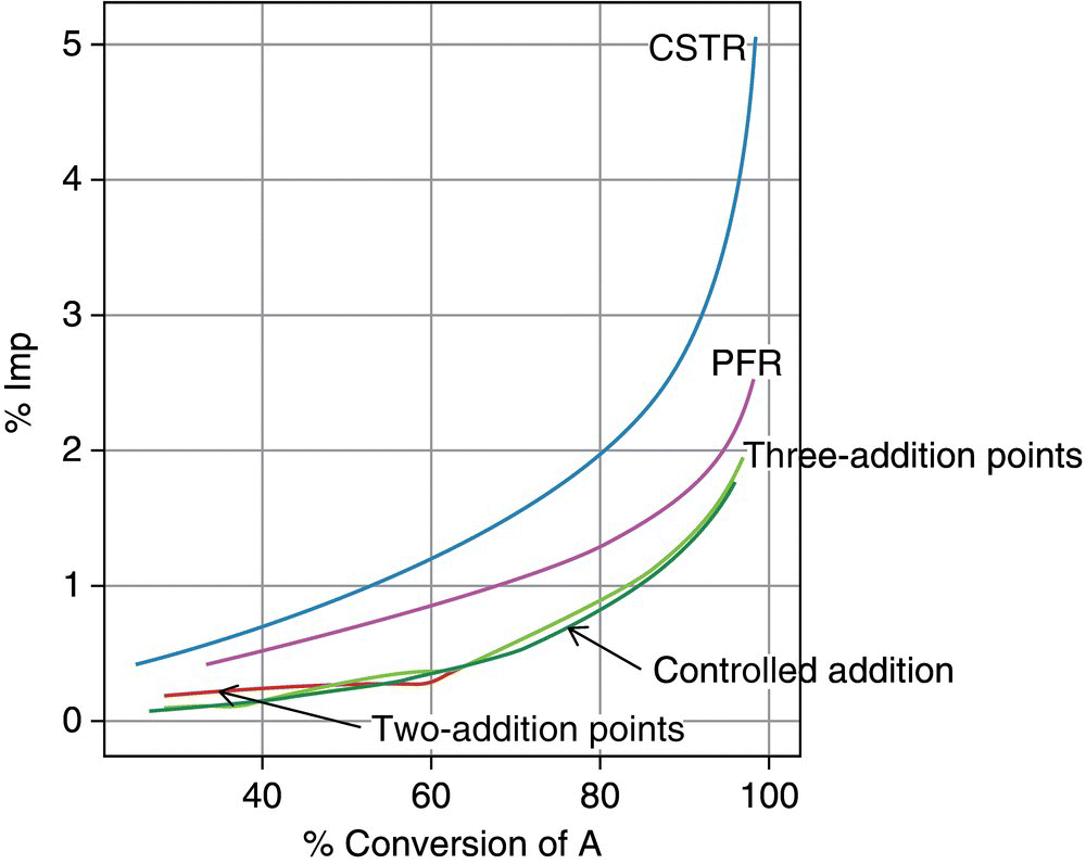
FIGURE 16.15 Impurity level vs. conversion for PFR, batch with controlled addition, 3 CSTRs with equal residence times, and PFR with multiple addition points along the length.
In this case, a controlled addition (semi‐batch) gives a lower impurity level than a PFR because it keeps the concentration of B lower. CSTRs give the highest level of impurities in this case because they are operating at steady‐state conditions with P and B together for longer times. B is at low levels, but P is always at high concentration levels, and contact time is 3 hours in the three CSTRs in series. The figure also shows two additional scenarios that begin to mimic batch with controlled addition in a PFR. Reagent B is added at multiple points along the PFR. The normal PFR has one addition point, which is at the inlet to the tube. The PFR with one side stream has two addition points, one at the inlet and one 1/3 of the way down the reactor length. Half of the reagent B feed solution was added at each location. The PFR with two side streams has three addition points. One is at the inlet, the second is at a distance 1/6 of the way down the reactor length, and the third is at a distance 1/3 of the way down the reactor length. Reagent B feed solution was added in three equal portions at the three locations. Interestingly, the impurity level in the PFR with multiple addition points matched batch reactor with controlled addition, even with only one side stream. Practically speaking, the cost of running a PFR with side streams is that another pump or control valve with mass flow control is needed for each additional side stream. This may be low cost compared to the benefit in yield and selectivity. Clearly, the numerical modeling is useful for reactor design and selection provided that the kinetics of the main reaction and of the unwanted side and series reactions are known. It is especially important when the impurities are difficult to reject and/or could be reactive downstream.
16.6 WHAT CAN BE DONE BATCH BEFORE RUNNING CONTINUOUS REACTION EXPERIMENTS?
Much of the experimental work to generate the data needed to develop a continuous flow process can actually be accomplished more quickly and efficiently in batch equipment. The impact of different reagents, solvents, and catalysts can often be run using less material in batch. In addition, batch experiments do not have the transitional waste produced in flow experiments to achieve steady state after changing an operational parameter. One may observe reaction characteristics in batch (such as solid precipitation) that will influence the eventual choice of flow reactor type or even advise when a flow process undesirable. Table 16.3 is a guide to what can be done batch to help design the continuous reaction before running continuous flow experiments.
TABLE 16.3 Batch Experimental Work That Can Inform Design for Flow
| Solubility | Try to make all reagent solutions in addition funnels or syringe pumps, i.e. no solid charges if possible. Solid precipitation in the continuous reactor is much easier to handle than a continuous slurry feed to the reactor. Establish homogeneous solution feeds |
| Measure solubility of reagents, products, intermediates, and by‐products | |
| Visual observation over time. If possible, observe changes in physical state throughout Monitor for solid precipitation or gas evolution at all extents of conversion during reaction. Solids sticking to the walls of the batch reactor indicate that fouling will likely occur if the reaction were run in flow | |
| If there are solids, are they sticky and clumpy or more like a well‐behaved crystallization? Use of a CSTR or slurry flow PFR is OK for well‐behaved solids but not for sticky clumpy solids | |
| CSTRs | If considering a CSTR, then batch‐on‐batch reactions can be run to mimic what would be expected in a CSTR. Run a batch reaction at minimum stir volume; then run another batch reaction on top of it. Is impurity profile better or worse for the second reaction? An intermittent flow CSTR can be mimicked by running a batch reaction, followed by a decant leaving a heel, followed by another batch, then decant with a heel, and so on. Test different heel volumes |
| Test the impact of order of addition. Coaddition of A and B versus controlled addition of A to B versus all‐at‐once addition of A and B (although all‐at‐once addition may be difficult to test batch). This will help to select between a CSTR (coaddition), intermittent flow CSTR (A to B), and PFR (all‐at‐once addition) | |
| Stability | Test the chemical stability of reagent solutions with time. Feed solutions should have a stability in excess of one week |
| What reagents, catalysts, and additives can be pre‐combined into a single feed, and which should be separate feeds for stability in the feed tank at room temperature? It is desirable to use as few feed streams as feasible to simplify the flow process | |
| Is the reaction stable to end‐of‐reaction conditions? Test for impurities versus time for extended hold times in the batch reactor. Watch for precipitation of solids during extended hold | |
| Impurities | Identify impurities and develop analytical methods from batch experiments |
| Monitor impurities versus time. Are they primarily late forming or early forming? If early forming, then consider using a CSTR. If late forming, then a PFR might be more advantageous | |
| Test the impact of temperature, pressure, stoichiometry, concentration, on rate, and impurities | |
| Test the impact of level of inertion and the impact of dissolved gases on impurity formation | |
| Test the impact of stripping during reaction versus operating with a sealed headspace. These impact the choice between a PFR designed for gas and liquid and liquid only | |
| Kinetics | Measure rates. Collect samples for conversion versus time data as standard practice. Quantitative conversion data is much more valuable than area % |
| Quantify kinetics of secondary reactions especially with respect to impurity profile | |
| Monitor concentration of intermediates over time | |
| Use of PAT for reaction monitoring and for model fitting to the rate profile curve. This provides the reaction rate and also proves a PAT tool to use when you run flow chemistry. Flow NMR is a valuable screening tool for kinetics because it gives quantitative conversion versus time with direct molar ratios | |
| Safety | Test materials of construction for corrosion and also impact on reaction |
| Do chemical reaction safety testing for heat of reaction: ARC, DSC, and RC1 | |
| Screening | If you plan to use a stirred tank because of solid precipitation, then try to find conditions that achieve complete conversion in 1 h or less in the batch reactor |
| In a PFR, if the reaction is a homogeneous solution at reaction temperature but not after cooling to ambient temperature, then you may be able to add in a diluting solvent at the exit of the PFR before cooling to keep solids from precipitating downstream from the reactor. Determine this in batch experiments first | |
| For reactions involving a homogeneous solution in the reactor or that are gas–liquid with only one liquid phase, then 12 h reaction time is acceptable in a PFR. In other words, find conditions that achieve complete conversion in about 12 h or less in the batch reactor | |
| Discreet variables (solvent, reagent, catalyst, ligand) are best scouted in batch; continuous variables (T, P, τ, and in some cases stoichiometry and concentration) may be best screened in flow | |
| Screen at high and low temperatures and at high pressures in batch reactions. Go more extreme in these process parameters than you would if you were developing a batch reaction for standard manufacturing equipment | |
| Think more broadly about solvent selection. One can operate far above the normal solvent boiling temperature by operating in a high pressure flow reactor. Solvents can be selected based on simplifying workup, greenness, and cost, in addition to yield and selectivity, even if the normal boiling point of the solvent is much lower than the desired reaction temperature, because PFRs enable running the reaction in superheated solvent | |
| You may be able to more easily perform the reaction in a high boiling solvent and then isolate the product from a low boiling solvent. Solvent exchange from a high to a low boiling solvent can be more efficient continuous than batch | |
| Initial route scouting should be done batch | |
| If you are running a gas–liquid reaction with a mixture of gases, like H2/CO, or O2/N2, test the impact of the feed gas stoichiometry | |
| Investigate large particle size catalyst. Reuse catalyst several times. Does activity decrease over time? Does metal leach? If not then consider a packed catalyst bed flow reactor | |
| Use the breathing autoclaves first if the reaction is an aerobic oxidation with dilute oxygen in nitrogen | |
| Test the impact of the reactor headspace volume. If there is advantage to zero headspace, then the reaction is a good candidate to utilize a PFR | |
| Investigate the effect of mixing rate | |
| Thermodynamics and fluid properties | Measure phase transition points for the reaction solution, i.e. boiling point, freezing point, and precipitation point |
| Measure the thermal expansion of the reaction mixture and the product mixture | |
| Measure densities of all feed and product solutions at room temperature. This is especially important if you will be pumping with a volumetric pump like a syringe or peristaltic |
16.7 WHAT IS DIFFICULT TO PREDICT FROM BATCH EXPERIMENTS?
Table 16.4 lists information that is best obtained in the actual flow chemistry experiments because it is difficult to predict from batch experiments.
TABLE 16.4 In Batch Experiments It Would Be Difficult to Predict Information About the Following
| Packed catalyst bed | If designing for a packed catalyst bed PFR, then catalyst life, i.e. number of reactor volume turnovers achievable with single catalyst charge, is best measured in flow |
| Localized equivalents of catalyst relative to dissolved reagents in a packed bed reactor can be orders of magnitude higher than with solids suspended in a stirred tank. The impact of this high catalyst loading is best tested in flow. The extremely high gas–liquid mass transfer rate of a trickle bed reactor is not feasible to duplicate in batch reaction experiments | |
The following should be probed in flow:
|
|
| Pressure, temperature, concentration, vapor–liquid flow conditions, and residence time to minimize problematic impurities and minimize catalyst deactivation over time are better tested in flow because it is difficult for batch reactions to predict impurity profiles in a continuous packed catalyst bed | |
| Flow regime should be tested in the continuous reactor (trickle, pulse, spray, or bubble). What are the gas and liquid linear velocities at the transition points from one flow regime to another? For example, if increasing flows in a trickle bed reactor, at what flow rates does the transition from trickle flow to bubble flow occur? | |
| Recycle | Effect of recycle on yield and impurity profile and impurity buildup in recycle loop over time |
| Fouling | Plugging and fouling issues and thus reliability over time for the flow process |
| Heat and mass transfer rates | Heat and mass transfer coefficients in tube reactors |
| Effect of fast heat‐up and cooldown times (on order of seconds) on yield, selectivity. Are yield and impurity profile sensitive to heat‐up time, cooldown time, and time at reaction temperature? These are easier to test flow than batch | |
| Extreme temperatures and reactions in supercritical fluids with short residence time, for example, Newman–Kwart thermal rearrangement in supercritical DME [23] and thermal BOC deprotection in supercritical THF [24] | |
| All‐at‐once stoichiometric reagent addition, i.e. PFR operating mode. It is especially difficult to measure batch for fast exothermic reactions, for example, cryogenic lithiation and coupling, because it could be difficult or impossible to maintain nearly isothermal reaction conditions with all‐at‐once addition batch | |
| PFR | Yield and impurity profile of organic azide formation reactions because of the need to run 100% liquid filled to avoid hydrazoic acid partition into the headspace [8] |
| Impurity profile for fast reactions in series with unstable intermediates, like cryogenic lithiation, coupling, and quench | |
| CSTR | Steady‐state yield and selectivity for Grignard formation reactions in a CSTR. The batch startup event with initiating agent like DIBAL or iodine may not be representative of steady‐state CSTR operation [25] |
| Reaction rates for extremely fast exothermic reaction like a Grignard formation. The reaction rate constants are more accurately measured by running a CSTR at steady state with incomplete conversion and calculating the rate constant from the CSTR design equation |
ACKNOWLEDGMENTS
Mark Kerr was the process chemist for the continuous Grignard formation reaction in the 100 L CSTR, and Sylvia Nwosu was the engineer on the scale‐up project. The third‐party CMO who did the scale‐up manufacturing work did an outstanding job and are largely responsible for the success of the project. Ed Deweese, Paul Milenbaugh, and Rick Spears of D & M Continuous Solutions constructed and operated the hydrogenation PFR system. Jake Remacle, Miguel Gonzales, Wei‐Ming Sun, and Nick Zaborenko developed the 73 L coiled tube PFR for hydrogenation, and the chemistry was designed and developed by Joel Calvin. We thank Bret Huff for initiating, leading, and sponsoring the continuous reaction design and development work at Eli Lilly and Company.
REFERENCES
- 1. (a) Malet‐Sanz, L. and Susanne, F. (2012). Continuous flow synthesis. A pharma perspective. J Med Chem 55 (9): 4062–4098.
(b) LaPorte, T.L. and Wang, C. (2007). Continuous processes for the production of pharmaceutical intermediates and active pharmaceutical ingredients. Curr Opin Drug Discov Devel 10 (6): 738–745.
(c) Wegner, J., Ceylan, S., and Kirschning, A. (2012). Flow chemistry: a key enabling technology for (multistep) organic synthesis. Adv Synth Catal 354 (1): 17–57.
(d) Mullin, R. (2007). Novartis and MIT study drug production. Chemical & Engineering News (8 October 2007), p. 10.
(e) Pellek, A. and Van Arnum, P. (2008). Continuous processing: moving with or against the manufacturing flow. Pharm Technol 9 (32): 52–58.
(f) Gutmann, B., Cantillo, D., and Kappe, C.O. (2015). Continuous‐flow technology: a tool for the safe manufacturing of active pharmaceutical ingredients. Angew Chemie Int Ed 54 (23): 6688–6728.
(g) Anderson, N.G. (2012). Using continuous processes to increase production. Org Process Res Dev 16 (5): 852–869.
(h) Hessel, V., Kralisch, D., Kockmann, N. et al. (2013). Novel process windows for enabling, accelerating, and uplifting flow chemistry. ChemSusChem 6 (5): 746–789.
(i) Baxendale, I.R. (2013). The integration of flow reactors into synthetic organic chemistry. J Chem Technol Biotechnol 88 (4): 519–552.
(j) Baxendale, I.R., Braatz, R.D., Hodnett, B.K. et al. (2016). Achieving continuous manufacturing: technologies and approaches for synthesis, workup, and isolation of drug substance May 20‐21, 2014 continuous manufacturing symposium. J Pharm Sci 104 (3): 781–791.
(k) Hartman, R.L., McMullen, J.P., and Jensen, K.F. (2011). Deciding whether to go with the flow: evaluating the merits of flow reactors for synthesis. Angew Chem Int Ed Engl 50 (33): 7502–7519.
(l) Mascia, S., Heider, P.L., Zhang, H. et al. (2013). End‐to‐end continuous manufacturing of pharmaceuticals: integrated synthesis, purification, and final dosage formation. Angew Chem Int Ed Engl 52 (47): 12359–12363.
(m) Scott, A. (2013). Pfizer adds biologics capacity, continuous processing in Ireland. Chem Eng News 91 (29): 9. - 2. (a) Webb, D. and Jamison, T.F. (2010). Continuous flow multi‐step organic synthesis. Chem Sci 1 (6): 675.
(b) McQuade, D.T. and Seeberger, P.H. (2013). Applying flow chemistry: methods, materials, and multistep synthesis. J Org Chem 78 (13): 6384–6389.
(c) Ahmed‐Omer, B., Barrow, D.A., and Wirth, T. (2011). Multistep reactions using microreactor chemistry. Arkivoc 4: 26–36.
(d) Grongsaard, P., Bulger, P.G., Wallace, D.J. et al. (2012). Convergent, kilogram scale synthesis of an Akt kinase inhibitor. Org Process Res Dev 16 (5): 1069–1081.
(e) Browne, D.L., Baumann, M., Harji, B.H. et al. (2011). A new enabling technology for convenient laboratory scale continuous flow processing at low temperatures. Org Lett 13 (13): 3312–3315.
(f) Fandrick, D.R., Roschangar, F., Kim, C. et al. (2011). Preparative synthesis via continuous flow of 4, 4, 5, 5‐tetramethyl‐2‐(3‐trimethylsilyl‐2‐propynyl)‐1, 3, 2‐dioxaborolane: a general propargylation reagent. Org Process Res Dev 16 (5): 1131–1140.
(g) Desai, A.A. (2012). Overcoming the limitations of lithiation chemistry for organoboron compounds with continuous processing. Angew Chem Int Ed 51 (37): 9223–9225. - 3. Kockmann, N. and Roberge, D.M. (2009). Harsh reaction conditions in continuous‐flow microreactors for pharmaceutical production. Chem Eng Technol 32 (11): 1682–1694.
- 4. (a) Baxendale, I.R., Braatz, R.D., Hodnett, B.K. et al. (2015). Achieving continuous manufacturing: technologies and approaches for synthesis, workup, and isolation of drug substance. May 20–21, 2014 continuous manufacturing symposium. J Pharm Sci 104 (3): 781–791.
(b) Anderson, N.G. (2012). Using continuous processes to increase production. Org Process Res Dev 16 (5): 852–869.
(c) Hessel, V., Kralisch, D., Kockmann, N. et al. (2013). Novel process windows for enabling, accelerating, and uplifting flow chemistry. ChemSusChem 6 (5): 746–789.
(d) Mascia, S., Heider, P.L., Zhang, H. et al. (2013). End‐to‐end continuous manufacturing of pharmaceuticals: integrated synthesis, purification, and final dosage formation. Angew Chem Int Ed 52 (47): 12359–12363. - 5. (a) Wegner, J., Ceylan, S., and Kirschning, A. (2012). Flow chemistry–a key enabling technology for (multistep) organic synthesis. Adv Synth Catal 354 (1): 17–57.
(b) Brocklehurst, C.E., Lehmann, H., and La Vecchia, L. (2011). Nitration chemistry in continuous flow using fuming nitric acid in a commercially available flow reactor. Org Process Res Dev 15 (6): 1447–1453.
(c) Brandt, J.C., Elmore, S.C., Robinson, R.I., and Wirth, T. (2010). Safe and efficient Ritter reactions in flow. Synlett (20): 3099–3103.
(d) Delville, M.M., Nieuwland, P.J., Janssen, P. et al. (2011). Continuous flow azide formation: optimization and scale‐up. Chem Eng J 167 (2): 556–559.
(e) Palde, P.B. and Jamison, T.F. (2011). Safe and efficient tetrazole synthesis in a continuous‐flow microreactor. Angew Chem Int Ed 50 (15): 3525–3528. - 6. Mastronardi, F., Gutmann, B., and Kappe, C.O. (2013). Continuous flow generation and reactions of anhydrous diazomethane using a Teflon AF‐2400 tube‐in‐tube reactor. Org Lett 15 (21): 5590–5593.
- 7. Dunn, P.J., Wells, A., and Williams, M.T. (eds.) (2010). Green chemistry in the pharmaceutical industry. Weinheim: Wiley.
- 8. Kopach, M.E., Murray, M.M., Braden, T.M. et al. (2009). Improved synthesis of 1‐(azidomethyl)‐3, 5‐bis‐(trifluoromethyl) benzene: development of batch and microflow azide processes. Org Process Res Dev 13 (2): 152–160.
- 9. Poechlauer, P., Colberg, J., Fisher, E. et al. (2013). Pharmaceutical roundtable study demonstrates the value of continuous manufacturing in the design of greener processes. Org Process Res Dev 17 (12): 1472–1478.
- 10. Mascia, S., Heider, P.L., Zhang, H. et al. (2013). End‐to‐end continuous manufacturing of pharmaceuticals: integrated synthesis, purification, and final dosage formation. Angew Chem Int Ed 52 (47): 12359–12363.
- 11. (a) Gutmann, B., Cantillo, D., and Kappe, C.O. (2015). Continuous‐flow technology: a tool for the safe manufacturing of active pharmaceutical ingredients. Angew Chem Int Ed 54 (23): 6688–6728.
(b) Anderson, N.G. (2012). Using continuous processes to increase production. Org Process Res Dev 16 (5): 852–869.
(c) Hessel, V., Kralisch, D., Kockmann, N. et al. (2013). Novel process windows for enabling, accelerating, and uplifting flow chemistry. ChemSusChem 6 (5): 746–789.
(d) Baxendale, I.R. (2013). The integration of flow reactors into synthetic organic chemistry. J Chem Technol Biotechnol 88 (4): 519–552.
(e) Baxendale, I.R., Braatz, R.D., Hodnett, B.K. et al. (2015). Achieving continuous manufacturing: technologies and approaches for synthesis, workup, and isolation of drug substance. May 20–21, 2014 continuous manufacturing symposium. J Pharm Sci 104 (3): 781–791. - 12. (a) Lee, S.L., O'Connor, T.F., Yang, X. et al. (2015). Modernizing pharmaceutical manufacturing: from batch to continuous production. J Pharm Innov 10 (3): 191–199.
(b) Allison, G., Cain, Y.T., Cooney, C. et al. (2015). Regulatory and quality considerations for continuous manufacturing. May 20–21, 2014 continuous manufacturing symposium. J Pharm Sci 104 (3): 803–812. - 13. White, T.D., Berglund, K.D., Groh, J.M. et al. (2012). Development of a continuous Schotten–Baumann route to an acyl sulfonamide. Org Process Res Dev 16 (5): 939–957.
- 14. May, S.A. and Johnson, M.D. (2013). Continuous processing to enable more efficient synthetic routes and improved process safety. Pharm Outsourcing 14 (5 API Supplement): 10–16.
- 15. (a) Levenspiel Octave, S. (1979). The Chemical Reactor Omnibook. Corvallis, OR: Oregon State University Book Stores.
(b) Levenspiel Octave, S. (1962). Chemical Reaction Engineering. An Introduction to the Design of Chemical Reactors. New York: Wiley.
(c) Fogler, H.S. (1999). Elements of Chemical Reaction Engineering, 3e. New Delhi: Prentice Hall PTR.
(d) Weber, W.J. and DiGiano, F.A. (1996). Process Dynamics in Environmental Systems. New York: Wiley. - 16. Johnson, M.D., May, S.A., Calvin, J.R. et al. (2012). Development and scale‐up of a continuous, high‐pressure, asymmetric hydrogenation reaction, workup, and isolation. Org Process Res Dev 16 (5): 1017–1038.
- 17. (a) McMullen, J.P. and Jensen, K.F. (2011). Rapid determination of reaction kinetics with an automated microfluidic system. Org Process Res Dev 15 (2): 398–407.
(b) Jensen, K.F., Reizman, B.J., and Newman, S.G. (2014). Tools for chemical synthesis in microsystems. Lab Chip 14 (17): 3206–3212.
(c) Chaudhari, R.V., Parande, M.G., Ramachandran, P.A. et al. (1985). Hydrogenation of butynediol to cis‐butenediol catalyzed by Pd‐Zn‐Caco3: reaction‐kinetics and modeling of a batch slurry reactor. AIChE J 31: 1891–1903.
(d) Makiarvela, P., Salmi, T., and Paatero, E. (1994). Kinetics of the chlorination of acetic‐acid with chlorine in the presence of chlorosulfonic acid and thionyl chloride. Ind Eng Chem Res 33: 2073–2083.
(e) Zaldivar, J.M., Molga, E., Alos, M.A. et al. (1996). Aromatic nitrations by mixed acid. Fast liquid‐liquid reaction regime. Chem Eng Process 35: 91–105. - 18. (a) May, S.A., Johnson, M.D., Braden, T.M. et al. (2012). Rapid development and scale‐up of a 1 H ‐4‐substituted imidazole intermediate enabled by chemistry in continuous plug flow reactors. Org Process Res Dev 16 (5): 982–1002.
(b) Levenspiel Octave, S. (1962). Chemical Reaction Engineering. An Introduction to the Design of Chemical Reactors. New York: Wiley. - 19. Process Systems Enterprise (1997–2016). gPROMS. www.psenterprise.com (accessed 14 October 2018).
- 20. Wehner, J.F. and Wilhelm, R.H. (1956). Boundary conditions of flow reactor. Chem Eng Sci 6 (2): 89–93.
- 21. (a) Braden, T.M., Johnson, M.D., Kopach, M.E. et al. (2017). Development of a commercial flow Barbier process for a pharmaceutical intermediate. Org Process Res Dev 21 (3): 317–326.
(b) Wong, S.‐W., Changi, S.M., Shields, R. et al. (2016). Operation strategy development for Grignard reaction in a continuous stirred tank reactor. Org Process Res Dev 20 (2): 540–550. - 22. Scale‐up Systems Limited (2011). Dynochem 2011 (4.0.0.0), Ireland. www.scale‐up.com (Accessed June 2015).
- 23. Tilstam, U., Defrance, T., Giard, T., and Johnson, M.D. (2009). The Newman−Kwart rearrangement revisited: continuous process under supercritical conditions. Org Process Res Dev 13 (2): 321–323.
- 24. May, S.A., Johnson, M.D., Braden, T.M. et al. (2012). Rapid development and scale‐up of a 1 H‐4‐substituted imidazole intermediate enabled by chemistry in continuous plug flow reactors. Org Process Res Dev 16 (5): 982–1002.
- 25. Kopach, M.E., Roberts, D.J., Johnson, M.D. et al. (2012). The continuous flow Barbier reaction: an improved environmental alternative to the Grignard reaction? Green Chem 14 (5): 1524–1536.