
42
USE OF PROCESS ANALYTICAL TECHNOLOGY (PAT) IN SMALL MOLECULE DRUG SUBSTANCE REACTION DEVELOPMENT
Dimitri Skliar, Jeffrey Nye,f and Antonio Ramirez
Product Development, Bristol‐Myers Squibb, New Brunswick, NJ, USA
42.1 INTRODUCTION
Reaction engineering is an essential component of quality risk management in pharmaceutical drug substance manufacturing. Identification of critical impurities, elucidation of reaction mechanisms leading to them, and characterization of reaction parameter space are key elements of robust and manufacturing‐ready chemical processes. Historically, chromatographic methods have been the analytical workhorse for monitoring chemical reactions throughout the pharmaceutical industry, as they provide unmatched sensitivity and specificity for a variety of organic compounds. However, one inherent shortcoming is the “off‐line” nature of the technique – samples must be collected and prepared prior to analysis, which may change the chemical nature of the analyte of interest. And while UPLC has dramatically shortened the time required for chromatographic separation, an inherent time delay exists between sampling and analysis.
Real‐time analytical tools provide an attractive complement to traditional chromatography by delivering a continuous stream of data from the direct interface with the reaction stream. Such tools are referred to as process analytical technology (PAT) analyzers, which can include simple univariate measuring devices such as temperature and pressure sensors but more commonly involve “in‐line” analyzers such as mid‐infrared (IR), near‐infrared (NIR), and Raman spectrometers. PAT analyzers provide real‐time information of chemical reactions by tracking the spectra of the molecules involved in the transformation.
Though the FDA [1] and EMEA definitions of PAT analyzers pertain to a manufacturing setting, these tools offer a number of benefits in laboratory development of chemical reactions as well. The exquisite time resolution associated to the capacity of collecting data points on the time scale of seconds allows for detailed kinetic analysis of complex reactions. Moreover, since these tools directly interface with the reaction stream, they enable the detection of reactive or short‐lived intermediates, which cannot be accurately identified via chromatographic methods. The in‐line nature also allows for analysis of hazardous systems, eliminating the requirement that an operator collects samples. In this manner, PAT analyzers provide improved safety when designing or optimizing processes involving highly toxic chemicals, reactions under pressure, or reactions at extreme temperatures. Finally, the fast acquisition time of PAT analyzers allows for timely response of processing conditions to reaction progress. This can enable feedback control when implementing fully developed processes and is a crucial component of flow reactions [2]. With these benefits in mind, significantly improved and user‐friendly experimental PAT units have become available for laboratory use, which have enabled facile experimentation on even very small scales, and have streamlined transfer of knowledge and methods to pilot and manufacturing scale. This chapter presents an overview of standard spectroscopy‐based PAT analyzers and their application to pharmaceutically relevant transformations. A number of case studies are chosen to illustrate both the enabling aspects of PAT in laboratory reaction development as well as their implementation in a manufacturing setting as part of a control strategy.
42.2 PAT METHODS
While the physics underlying the various spectroscopic techniques discussed in this chapter varies, the general principles of implementing PAT are common to all of them. Light is directed from a source within the spectrometer through a conduit into a probe that is immersed in the reaction stream of interest. Analyzed light, be it an absorption spectrum or scattered photons, is then directed back to a detector, processed, and presented as a spectrum that changes with time as the reaction progresses. Spectral data can be processed and interpreted in a variety of ways, both quantitative and qualitative. Table 42.1 lists the wavelength and frequency ranges for common analytical techniques based on electromagnetic radiation [3]. Ultraviolet–visible, NIR, mid‐IR, and Raman spectroscopies are the four most common methods used for reaction monitoring and analysis. These techniques cover the wavelength range of the electromagnetic spectrum between 180 nm and 300 μm (see highlighted rows in Table 42.1).
TABLE 42.1 Spectroscopic Techniques Based on Electromagnetic Radiation
| Spectroscopy Type | Wavelength Range | Wavelength Range (cm−1) | Type of Quantum Transition |
| Gamma‐ray emission | 0.005–1.4 Å | — | Nuclear |
| X‐ray absorption, emission, fluorescence, and diffraction | 0.1–100 Å | — | Inner electron |
| Vacuum ultraviolet absorption | 10–180 nm | 1 × 10⁶ to 5 × 10⁴ | Bonding electrons |
| Ultraviolet–visible absorption, emission, and fluorescence | 180–780 nm | 5 × 10⁴ to 1.3 × 10⁴ | Bonding electrons |
| Near‐infrared and mid‐infrared absorption and Raman scattering | 0.78–300 μm | 1.3 × 10⁴ to 33 | Rotation and vibration of molecules |
| Microwave absorption | 0.75–3.75 mm | 13–27 | Rotation of molecules |
| Electron spin resonance | 3 cm | 0.33 | Spin of electrons in a magnetic field |
| Nuclear magnetic resonance | 0.6–10 m | 5 × 10⁻² to 1.3 × 10⁻³ | Spin of nuclei in a magnetic field |
A typical in‐line instrument setup for use in laboratory consists of a probe that can be inserted into a reaction vessel, a spectrometer, and a computer interface where data can be processed (see Figure 42.1). Standard probe diameters allow for utilization of vessel sizes ranging from several milliliter vials all the way to multi‐liter scale reactors (see Figure 42.2a and b). For improved and automated analysis, a variety of instruments are available that combine spectroscopic collection with process parameter monitoring (such as temperature, pressure, agitation speed, etc.) in one package (see Figure 42.2c).

FIGURE 42.1 Schematic of laboratory setup for in‐line spectroscopic monitoring.
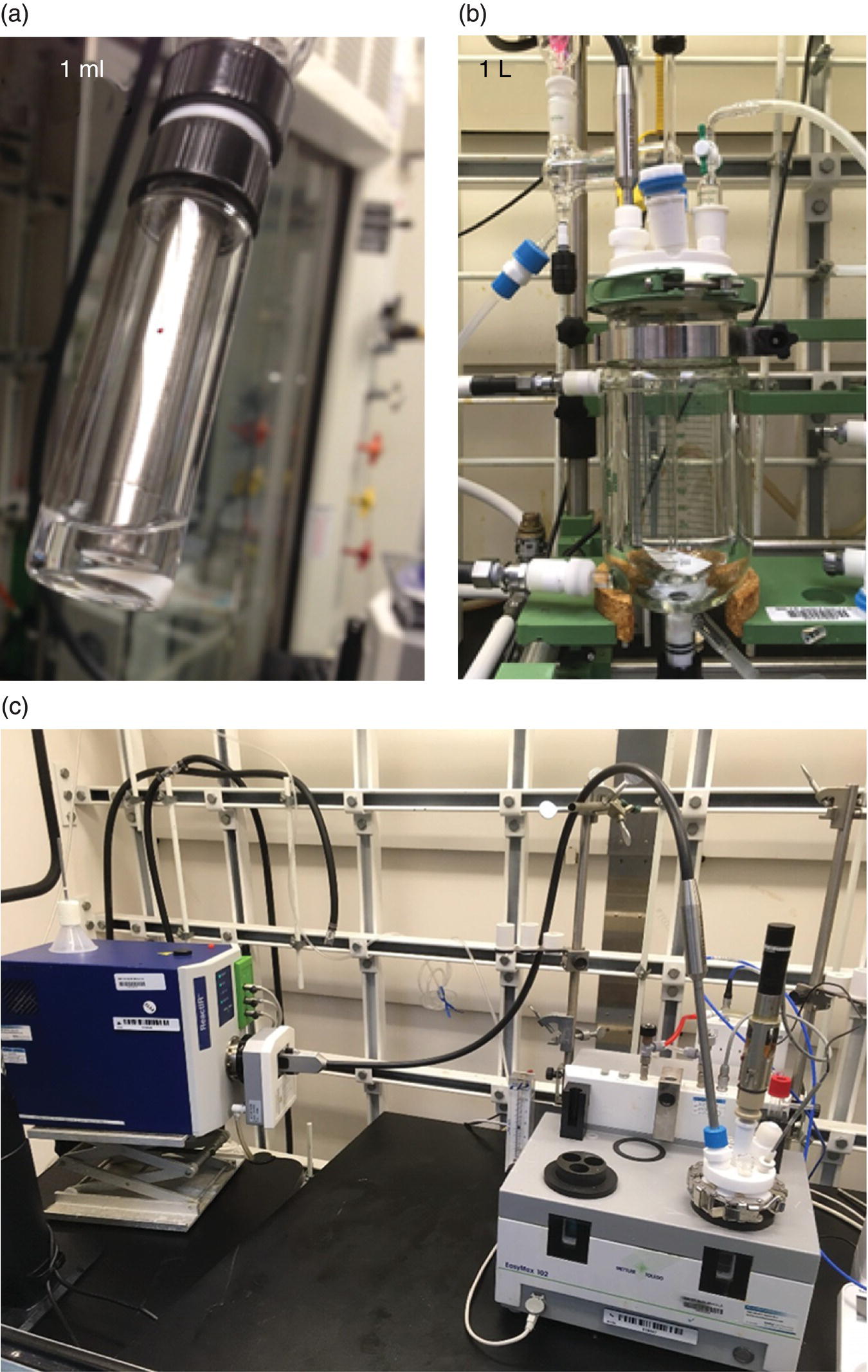
FIGURE 42.2 (a) Spectroscopic probe inserted into 4 ml vial. (b) Spectroscopic probe inserted into 1 L reactor. (c) Mettler Toledo ReactIR 45 M instrument coupled with EasyMax reactor setup.
Several probe configurations are suitable for scale‐up implementation of PAT. The reaction mixture can be analyzed by inserting a probe through a reactor port, a bottom valve, or a recirculation loop (Figure 42.3). Commercially available instruments for the spectroscopy types discussed in this chapter can be utilized on scale in these configurations.
FIGURE 42.3 Schematic of different possible PAT configurations for implementation on scale.
42.2.1 Mid‐infrared Spectroscopy
IR spectroscopy examines molecular vibrations based on the absorption of light in the mid‐IR region of the electromagnetic spectrum (~400–4000 cm−1). As the IR absorption bands are often unique to the vibrational modes of chemical functional groups, IR spectroscopy provides a high degree of structural specificity in the analysis of liquids, solids, and gases and has long been used by analytical chemists in structural determination of unknown materials. The enabling technology underlying most IR spectrometers is the Michaelson interferometer, a common optical assembly that uses light interference to measure distances in wavelength units. IR light is transmitted from a source through a beam splitter and movable mirror; after interaction with the sample, an interferogram is detected and then converted to a true absorption spectrum by Fourier transform. Hence the technique is commonly known as Fourier transform infrared spectroscopy (FTIR).
A key difference in FTIR spectrometers used for real‐time analysis relative to standard benchtop units is the configuration of the optical element that transmits light from the spectrometer to the interface with the reaction stream. Traditional benchtop instruments measure IR absorption through a fixed length of sample in a transmission mode. In contrast, online measurements primarily employ a sampling element based on attenuated total reflectance (ATR) (Figure 42.4). In ATR measurements, light is transmitted through a solid material and reflected on the surface in contact with the sample before being sent back to the detector. This reflection establishes an evanescent wave that penetrates less than 2 μm into the sampled medium. Thus the ATR element enables in situ monitoring of the reaction being analyzed with zero sample preparation. ATR materials are chosen for low absorbance and high index of refraction, but as they are directly immersed in reaction streams, chemical inertness is a requirement. Diamond is frequently the material of choice, as it exhibits good IR transmission and is chemically inert to the wide range of chemistries employed in chemical development. Moreover, diamond is very hard, resists abrasion by solid particles, and is stable across a wide range of temperatures and pressures. One drawback is that diamond strongly absorbs IR radiation in the 1900–2300 cm−1 region, which overlaps with vibrational modes corresponding to triple and cumulated double bonds. Silicon is an alternative ATR element that provides high sensitivity across the IR spectrum and is thus ideal for monitoring reactions involving azides, acetylenes, carbon dioxide, etc. However, silicon is less chemically resistant, particularly to strong aqueous bases. Table 42.2 summarizes the physical properties of the materials generally used in ATR elements.

FIGURE 42.4 Attenuated total reflection sampling element.
TABLE 42.2 Materials Generally Used in ATR Elements
| Material | Spectral Range (cm−1) | Refractive Index | Depth of Penetration (μm) |
| Diamond | 4 500–2 500 1667–33 |
2.4 | 1.66 |
| Si | 8 300–1 500 360–70 |
2.37 | 1.73 |
| Ge | 5 500 | 4 | 0.65 |
| KRS‐5 | 20 000–400 | 2.37 | 1.73 |
| ZnSe | 20 000–650 | 2.4 | 1.66 |
An important challenge of PAT tools that incorporate ATR elements is the difficulty of transmitting light from the spectrometer to the sampled medium. Housing the ATR element in a metal probe, usually Hastelloy for its chemical inertness, facilitates light transmission to the reaction medium as well as the adequate ruggedness to withstand the breadth of chemical environments used in chemical development (strong acids and bases, very high or low temperatures, high pressure, etc.). In early FTIR instruments, the probe and the spectrometer were connected by a hollow light path with a series of adjustable mirrors to focus the IR laser beam to the probe. This system provides high performance and low attenuation across the spectrum, but achieving proper alignment of the probe requires a good level of expertise. A more robust, user‐friendly technology is the use of polycrystalline silver halide fibers, which provide a flexible connection between the probe and the spectrometer. Compared with probes with mirrored ends, fiber‐optic conduits can be aligned in a straightforward manner and display a lower sensitivity to movement and vibration. Since light attenuation through fiber optics increases with length and can be affected by conduit curvature, limitations exist on the physical size and configuration of the fibers, with typical fiber lengths being less than 3 m. One other consideration for the use of FTIR spectroscopy is that water strongly absorbs in the IR region. While this does not totally preclude the technique’s used in aqueous systems [4], it can make analysis difficult as many important regions of the spectrum may be obscured. In general, for solvents with absorptions that overlap with the analyte bands, adequately scaled solvent subtraction techniques [5] may facilitate reaction monitoring. When solvent subtraction is not suitable, other chemometric treatments such as principal component analysis (PCA), partial least squares (PLS) regression, principal component regression (PCR), or multiple linear regression (MLR) may be used to deconvolute reaction mixtures [6]. Figure 42.5 displays the IR transmission bands for solvents commonly used in chemical reactions. In addition to monitoring reactions, FTIR probes are routinely used to monitor crystallizations as the short penetration depth into the sample allows for supersaturation studies [7].

FIGURE 42.5 Infrared transmission for typical solvents used in chemical reactions. Dark regions with less than 50% transmission represent bands where analyte monitoring may require solvent subtraction.
42.2.2 Raman Spectroscopy
Raman spectroscopy probes molecular vibrations and rotations in the 100–3000 cm−1 frequency range. It is considered a complimentary technique to mid‐IR spectroscopy that analyzes the wavelength shifts associated to Raman scattering. When a sample is excited with monochromatic light, a small portion of the scattered radiation undergoes quantized changes in frequency that result in vibrational and rotational transitions. The Raman effect accounts for the new frequencies in the spectrum of the monochromatic light and is reported in “Raman shift” away from the monochromatic light source: Δν = ν± − (ν± ± ν1) = ±ν1, which is independent on the frequency of the monochromatic light, ν±.
Whereas IR absorption only occurs when the excited vibrational mode induces a change in dipole moment of the molecule, Raman scattering relies on a change in the molecule’s dipole polarizability – the temporary distortion of the electron density around bonds. Hence, a given vibrational mode may be “Raman active,” “IR active,” or both, and Raman spectra and IR spectra can be very different for a given molecule. For example, Raman spectroscopy can detect symmetric vibrations in diatomic molecules such as chlorine, oxygen, etc., whereas IR spectroscopy cannot. In a standard Raman spectrometer, monochromatic light from a laser is directed to a probe immersed in a reaction stream, where it interacts with the analyte. The scattered photons are then returned to the spectrometer and passed through a series of optical filters selected to exclude the wavelength of the laser itself – the majority of the light returning to the spectrometer will be Rayleigh scattered and thus be the same as the excitation wavelength. The strength of the Raman effect depends on the excitation wavelength and is dramatically increased at high excitation frequencies. Ideally, a lower wavelength light source will provide a stronger Raman spectrum. In practice, however, many samples will fluoresce when irradiated with low wavelength light. This fluorescence overwhelms the Raman scattered photons, making spectral interpretation difficult or impossible. Most commercial laboratory Raman instruments use one of three readily available laser lines, 532, 785, or 1000 nm. Among these, the 785 nm wavelength is the most common, as it provides a good balance between Raman intensity and low fluorescence in reaction systems relevant to pharmaceutical development. It should be noted that ambient light collected by the probe will also be detected and interferes with Raman spectra, so quantitative analysis requires that samples be protected from stray light sources.
Like FTIR probes, Raman probes generally consist of an optical window at the end of a Hastelloy pipe. The optical elements of a Raman probe are not ATR based, but instead rather focused into the reaction sample a few millimeters away from the probe tip. Many materials can be used for the window, including diamond, quartz, fused silica, and sapphire. The latter is the most common material because it offers a suitable arrangement of chemical inertness, strength, and availability. Since glass is Raman inactive, Raman probes can be fit with long working distance optics that enable indirect or noncontact measurement; samples can be analyzed through the glass wall of a vial, instead of immersed directly in the reaction stream. One key advantage of Raman spectroscopy over IR is that light is sent from the laser source to the immersed probe via standard optical fiber. The low attenuation along these fiber runs allows for physical separation between probe and spectrometer of up to hundreds of meters, enabling remote analysis and easing implementation in crowded laboratories and processing facilities. Since water is Raman inactive, it is an excellent technique for analyzing biotransformation streams such as fermentations.
42.2.3 Near‐infrared (NIR) Spectroscopy
NIR spectroscopy is an effective PAT tool that has found wide application in process development, quality control, and raw material testing [8]. The NIR region of the spectrum extends from the upper wavelength end of the visible region at 770–2500 nm (4000–13 000 cm−1) [9]. NIR absorption bands represent overtones or combinations of fundamental vibrational bands corresponding to the 1700–3000 cm−1 region. Chemical bonds that link a hydrogen atom to a heavy atom display vibrational transitions in this region and constitute the foundation of the widespread use of NIR to monitor molecules containing C─H, N─H, O─H, or S─H moieties. Due to the overtone nature of the vibrations, NIR spectroscopy is not suited for structural elucidation or identification of compounds, but is well qualified to perform quantitative analysis aided by chemometric techniques. Nevertheless, despite the complexity of NIR spectra, wavelength–structure correlations that can be used for guidance in qualitative analysis have been tabulated (Table 42.3) [10]. In addition to in situ monitoring of chemical processes, NIR spectroscopy has been used in a variety of fields including medical diagnostics, food quality control, and atmospheric chemistry. Typical instruments available for reaction monitoring are both benchtop off‐line units, capable of analyzing solids or liquids, and in‐line fiber‐coupled probes for direct analysis in a reactor setting.
TABLE 42.3 Wavelength–Structure Correlations for NIR Active Functional Groups
| Wavelength (nm) | Wavenumber (cm−1) | Assignment |
| 2 500 | 4 000 | Combination S─H stretch |
| 2 200–2 460 | 4 545–4 065 | Combination C─H stretch |
| 2 000–2 200 | 5 000–4 545 | Combination N─H stretch; combination O─H stretch |
| 1 620–1 800 | 6 173–5 556 | First overtone C─H stretch |
| 1 400–1 600 | 7 143–6 250 | First overtone N─H stretch; first overtone O─H stretch |
| 1 300–1 420 | 7 692–7 042 | Combination C─H stretch |
| 1 100–1 225 | 9 091–8 163 | Second overtone C─H stretch |
| 1 020–1 060 | 9 804–9 434 | Combination S=O stretch |
| 950–1 100 | 10 526–9 091 | Second overtone N─H stretch; second overtone O─H stretch |
| 850–950 | 11 765–10 526 | Third overtone C─H stretch |
| 775–850 | 12 903–11 765 | Third overtone N─H stretch |
| 600–700 | 16 667–14 286 | Combination C─S stretch |
| 450–550 | 22 222–18 182 | Combination S─S stretch |
42.2.4 Ultraviolet–Visible Spectroscopy
Ultraviolet–visible (UV‐Vis) spectroscopy analyzers measure the absorption of a sample in the mid‐ultraviolet to visible region of the electromagnetic spectrum that arise from electronic transitions (~200–700 nm, 50 000–14 000 cm−1). While lacking the chemical specificity of the techniques discussed above, it is commonly used to monitor liquid phase reactions due to its simplicity, sensitivity, and time resolution [11]. Despite spectral overlap, absorbance changes occurring during the reaction can be tracked and assigned to specific components with the aid of calibrated standards, chemometric techniques, or both. Moreover, analysis of the isosbestic points can help elucidate the number of absorbing species and lend support to mechanistic hypotheses [12]. A variety of sampling technologies are available for online and off‐line analysis, with both transmission and ATR‐based interfaces. UV‐Vis is commonly used for analysis of “colorful” compounds such as transition metal complexes [13] and highly conjugated molecules [14]. In the same way as other spectroscopic methods, the absorbance of the reaction solvents can interfere with the absorbance of the analytes, and lower wavelength cutoff limits below which solvent absorbance is excessive must be considered (Table 42.4). Since pharmaceutical processes are typically run at high concentrations in solvents that absorb UV light, care must be taken to avoid quantitative analysis in high‐absorbing regions of the spectrum by reducing path length in transmission mode or focusing on longer wavelengths.
TABLE 42.4 Lower Cutoff Wavelength Limits for Solvents Commonly Used in Chemical Reactions
| Solvent | UV Cutoff (nm) |
| Water | 191 |
| Methanol | 203 |
| Isopropyl alcohol | 205 |
| Acetone | 330 |
| Acetonitrile | 190 |
| Ethyl acetate | 256 |
| N,N‐Dimethylformamide | 268 |
| N‐Methylpyrrolidone | 285 |
| Tetrahydrofuran | 215 |
| tert‐Butyl methyl ether | 210 |
| Dichloromethane | 232 |
| 1,2‐Dichloroethane | 228 |
| n‐Heptane | 200 |
| Toluene | 284 |
42.2.5 Spectroscopy Interpretation (IR, Raman)
Complementing the observation of spectral differences detected during the course of a reaction with sound structural characterization can provide insight into reaction mechanisms. Spectral interpretation handbooks and databases are available in a number of online and printed resources [15],1 and most contemporary software packages provide approximate functional group assignments for the data collected.2 In general, this information should be helpful for a scientist to be able to assign characteristic peaks to a species one expects to observe in a particular reaction. For more accurate predictions of vibrational modes for a compound of interest, quantum mechanical packages such as Gaussian can be utilized [16].
42.3 PAT APPLICATION IN PHARMACEUTICAL REACTION ENGINEERING
42.3.1 General Reaction Types
Table 42.5 provides a summary of literature reports for common reaction types with their associated functional group transformations in the mid‐IR region. The abundance and diversity of the reactions explored with in situ spectroscopy methods speaks to the value of PAT to advance the design, implementation, and characterization of chemical processes.
TABLE 42.5 Spectroscopically Active Reaction Types Relevant to Pharmaceutical Reaction Development
| Reaction | Starting Material Characteristic Functional Group and Corresponding Vibrational Frequency (cm−1) | Product Characteristic Functional Group and Corresponding Vibrational Frequency (cm−1) |
| Nitroaromatic hydrogenation [17] | Ar─NO2 (1530)a | [Ar─NH─OH (3310)]b Ar─NH2 (3380) |
| Methyl nicotinate hydrogenation [18] | Pyr‐3‐CO2Me (1305, 1720) | Pip‐3‐CO2Me (1660) |
| Pyrazine hydrogenation [19] | Pyrazine (1675) | [Dihydropyrazine (1660)] Piperazine (1600) |
| α,β‐Unsaturated carboxylic acid [20] hydrogenation | RR′C=CH─CO2H.TMG (1625) | RR′CHCH2─CO2H.TMG (1625) |
| Grignard formation [21] | Ar─I | Ar─Mg (1035, 880) |
| 3‐Bromoquinoline Br‐metal exchange [22] | Bu3MgLi (700, 735) | Ar3MgLi (1270, 1335) ArMgBr (1260) Ar2Mg (1075) ArLi (1065, 1255) |
| ortho‐Lithiation [23] | Ar─H (1520) | ArLi (1420) |
| Lithiation of 3,5‐dichloropyridine [24] | 3,5‐diCl‐Pyr‐H (1110, 1010, 885, 810, 695) | 3,5‐diCl‐Pyr‐Li (753, 1007, 1140) |
| Aryl carbamate ortho‐lithiation [25] | R2NCO2Ar (1720) | R2NCO2ArLi (1660) |
| Grignard quench with CO2 [26] | CO2 (2340) | [RC=C─COMgCl (1650–1500)] |
| Acetylide addition to aldimine [27] | R─C(H)=N─R′ (1670) | [R─C(H)=N─R′─BF3] (1713) |
| Acetylide addition to Weinreb amide [28] | RCON(OMe)Me (1681 in pentane; 1663 in THF) | RCOR′ (1670, after quench) |
| Benzaldimine formation with LiHMDS [29] | ArCOH (1700) | ArC=N─TMS (1655) |
| Ester enolization [30] | R2CHCO2t‐Bu (1730) | R2C─CO2(Li)t‐Bu (1645–1665) |
| Oxazolidinone enolization [31] | R─CH2CO─Ox (1800) | R─CHCO(K)─Ox (1740–1715) |
| Sultam enolization [32] | RCH2CONRSO2R* (1695) | RCHLiCONRSO2R* (1620) |
| Formamide deprotonation [33] | HCONH2 (1710) | HCONHNa (1580) |
| Benzoic acid methylation [34] | PhCO2H (1700) | PhCO2Me (1725) [35], CH2N2 (2100) |
| Carboxylic acid to acid chloride [36] | R─CO2H (1710) | R─COCl (1805) |
| Carboxylic acid to acid chloride [37] | Ar─CO2H (1690) | Ar─COCl (1745, 1770) |
| Acid chloride to ketene [38] | RR′CHCOCl (1790) | RR′C=C=O (2200) |
| Acid chloride to ketene [39] | ArCH2COCl (1800) | ArHC=C=O (2330) |
| Modified Arndt–Eistert reaction [34] | ArCOCl (1775), CH2N2 (2100) | [ArCOCHN2 (2090)], CH2N2 (2100) |
| Amide bond formation with CDI [40] | ArCOImidazole (1790) | — |
| Curtius rearrangement to carbamate [18] | — | [RCON3 (1710)] RNCO2R (1725) |
| Aldol reaction [41] | H2C(OR)=CH(OR)OSiMe3 (1670) | [H2C(OR)=CH(OR)OBu4N (1625)] [H2C(OR)=CH(OR)OCuLn (1690, 1550)] R′CHOXC(OR)=CH(OR)OBu4N (1730) |
| Azide–alkyne cycloaddition [42] | Pyrimidinone (1680) | C=C triazole (1625) C=N, N=N triazole (1235) |
| Baeyer–Villiger oxidation [43] | RCOR | [ArCO3H (1165)], [peroxide Int (950)] |
aFrequency numbers rounded to the closest frequency within 5 cm−1 intervals.
bStructures in brackets represent reaction intermediates.
42.3.2 PAT Application in Complex Reaction Systems
The analysis of transformations involving reactive intermediates or multiphase media often presents a challenge for conventional off‐line analytical techniques (e.g. HPLC, GC, NMR). During process development and plant execution of such processes, utilization of in situ spectroscopic methods offers a significant advantage from accuracy, time of analysis, and progress monitoring perspectives.
Off‐line techniques are often destructive for reactive intermediates and may not be able to detect the high‐energy species due to their thermal or chemical instability (Figure 42.6a). While the addition of a derivatization step may facilitate conventional analysis, reproduction of the intermediate concentrations demands an innocuous sampling and a derivatization reaction that is viable, quantitative, and significantly faster than the reaction being monitored. Similarly, representative sampling can be difficult for heterogeneous reactions where multiphasic mixtures (e.g. solid–liquid) are present (Figure 42.6b). A common off‐line approach to measure analyte concentration in slurries involves sampling the slurry, filtering out the solids, and then performing the analysis using chromatographic or spectroscopic methods. Immersion probes can simplify this measurement by using direct detection since the ATR element is in close contact with the liquid phase and the interference from the solids is generally inconsequential [44].
FIGURE 42.6 Schematic illustration of reactions where PAT offers significant advantage over conventional techniques.
For pressurized reactions the use of in‐line spectroscopy can be crucial, as it eliminates the disturbance to the system associated with conventional sampling (Figure 42.6c). For example, sampling a catalytic hydrogenation under pressure often leads to modification of the reaction conditions due to exposure of the reaction mixture to non‐inert conditions, changes in composition, or variations in the partial pressure of hydrogen upon reaction restart. The ability to perform real‐time analysis using in‐line FTIR or at‐line NIR has been exploited to control selectivities in hydrogenations that afford a mixture of products [45]. Table 42.6 provides a brief summary of the benefits offered by PAT tools relative to conventional off‐line analysis methods.
TABLE 42.6 Benefits of PAT in Complex Reaction Systems
| “Standard” Analytical Techniques | Spectroscopy‐based Techniques |
| Reaction can be disturbed due to physical sampling | No physical sampling necessary |
| Unstable intermediates could be undetectable | Enable continuous monitoring of reactive intermediates |
| Long analysis time | Short analysis time that enables real‐time control |
42.4 CASE STUDIES
The case studies that follow highlight the use of PAT tools in complex reaction systems. They cover examples of the application of PAT to establish in‐process controls (IPCs), the description of method development, and the method implementation in a production setting.
42.4.1 Case Study 1: Control of Ammonia Content in Solution Using NIR Spectroscopy
Consider the chemical transformation depicted in Figure 42.7, where a pharmaceutical intermediate is synthesized via a reductive amination that involves the use of gaseous reagents under pressure [46]. The reaction is performed in two steps: (i) ketone ammonolysis by reaction with ammonia to form an intermediate ketimine and (ii) heterogeneous catalytic hydrogenation of the ketimine intermediate to give primary amine.
FIGURE 42.7 Reductive amination process.
In general, for reactions conducted under pressure where dissolved gas is present in significant amounts, it is important to design a robust purging protocol. Ensuring the solution is free of gas in downstream processing is necessary to guarantee safe handling and emissions controls. In this particular case, residual ammonia from the ammonolysis part of the process negatively impacted the hydrogenation step due to its correlation with increased levels of impurity and ammonia off‐gassing that complicated the charge of Pd/Al2O3 catalyst. During the first kilo‐scale implementation of the process, ammonia was removed from solution through a sequence of nitrogen purges. Due to inability to continuously subsurface sparge with nitrogen in the reaction vessel and high ammonia solubility in MeTHF (>1 mol/L), a large number of purge cycles needed to be implemented. Each purge cycle consisted of the following steps: venting of headspace to atmospheric pressure with agitation turned off, nitrogen introduction into the headspace to 1–2 psig, and agitation of solution for several minutes until pressure stabilization (i.e. a new ammonia liquid–vapor equilibrium was established), which was then followed by stopping of the agitator and venting of the headspace gas to a scrubber. This operation helped reduce headspace pressure close to atmospheric and enabled the charge of solid Pd/Al2O3 catalyst for the subsequent hydrogenation. Figure 42.8 depicts the pressure profile during the purge of residual ammonia for a representative reaction executed in a 20 L reaction vessel. Table 42.7 summarizes the impurity levels observed at different process stages in the three batches executed during the scale‐up campaign.
FIGURE 42.8 Headspace pressure during ammonia removal through nitrogen purges.
TABLE 42.7 Levels of Impurity Observed in the Reductive Amination
| Batch | Input (kg) | Level of Des‐halogenation Impurity in Process Stream Following Ammonolysis Completion (HPLC %) | Impurity in Process Stream Following Pd/Al2O3 Filtration (HPLC %) | Impurity in Isolated Cake (HPLC %) |
| 1 | 1.8 | <0.05 | 0.36 | 0.32 |
| 2 | 1.9 | <0.05 | 0.47 | 0.47 |
| 3 | 1.9 | <0.05 | 0.50 | 0.43 |
The impurity formed during filtration of the Pd/Al2O3 catalyst, following hydrogenation completion. Moreover, further investigations demonstrated that impurity formation rates were accelerated by increasing levels of residual ammonia. Interestingly, such high levels of impurity were never observed in laboratory experiments prior to scale‐up. Whereas filtration times are on the order of minutes in the laboratory, typical filtration times for plant‐scale hydrogenations (~1000 L) are on the order of hours. Therefore, implementing a control strategy that established acceptable ammonia levels in post‐ammonolysis stream to prolong post‐hydrogenation stream stability had to be considered. Evaluation of multiple spectroscopic techniques for detection of key reaction components is a good general practice when facing a new chemical transformation in the context of PAT development. In‐line or at‐line testing of reaction components in the solvent system of interest or reaction matrix allows to quickly assess if a particular technique has specificity for the compounds of interest. Figures 42.9 and 42.10 show, respectively, FTIR and NIR spectra of the reaction components. Inspection of the FTIR spectra in the 1500–1800 cm−1 region indicated that the carbonyl band of the starting material at approximately 1700 cm−1 is well separated from bands of other species and suggested that FTIR was well suited for monitoring the ammonolysis. Indeed, in situ FTIR monitoring enabled the rapid collection of kinetic information and characterization of the reaction parameter space with respect to conversion in the early stages of reaction development (Figures 42.11 and 42.12). For reaction times on the order days, the reaction required an ammonia pressure greater than 30 psig and excess of titanium tetra‐isopropoxide. Alternative methods to monitor the pressurized reaction were limited by frequency of sampling, safety, and moisture sensitivity. Unfortunately, due to overlap of amine‐containing functional groups in the product and ammonia in solution, quantitative determination of ammonia content with FTIR at low levels proved challenging.

FIGURE 42.9 FTIR spectra of various mixtures of reaction components.

FIGURE 42.10 NIR spectra of various mixtures of reaction components.
FIGURE 42.11 Ammonolysis reaction progress versus ammonia pressure.
FIGURE 42.12 Ammonolysis reaction progress versus Ti(OiPr)4 equivalents.
As presented in Figure 42.10, examination of the overlaid NIR spectra of starting material, imine intermediate with and without ammonia, and product indicated that NIR offers excellent specificity with respect to ammonia content, which appears as a strong peak at approximately 5000 cm−1. Having established that the characteristic peak of ammonia is well separated from other reaction components, the next step in method development was to construct the calibration curve. Although the off‐line measurement of a standard ammonia solution could potentially be employed with success, several drawbacks of such approach became apparent. Depending on a particular set of reaction conditions, the range of ammonia concentrations that needed to be spectroscopically characterized could only be achieved at pressures above atmospheric. Conversely, the need to detect low levels of ammonia made availability of standard solutions impracticable. In addition, due to the gas–liquid equilibrium nature of the dissolution process, the dependence of ammonia concentrations on headspace pressure and solution handling could introduce significant error during the calibration. Using in‐line spectroscopic measurements in the calibration eliminated these uncertainties. Figure 42.13 shows a schematic laboratory setup that utilizes a pressure vessel equipped with a supply line of gaseous ammonia, an NIR probe, and a pressure gauge. Using this setup, a simple protocol was devised to dissolve a known amount of gas in the reaction solvent. First, the reactor headspace was pressurized to a known value Po while the agitator was turned off. Second, the gas supply was turned off, and the agitator activated until an equilibrium pressure Pf at which a constant gauge reading was achieved. Using ideal gas law, namely, ![]() , allows to determine the number of moles of ammonia dissolved in solution for each such operation. Repeating this sequence several times (Figure 42.14) affords the calibration curve shown in Figure 42.15, where ammonia concentration is proportional to ammonia NIR peak height. In this particular case, the ammonia peak at approximately 5000 cm−1 was normalized relative to the MeTHF solvent peak. Development of the analytical method for in situ ammonia detection enabled conduction of laboratory stability studies for post‐hydrogenation streams of variable ammonia content. It was established that ammonia concentrations lower than 0.1 M afforded extended multi‐day stream stability. NIR IPC for residual ammonia concentrations lower than 0.1 M was set in place at the end of the ammonolysis reaction. Implementation of this spectroscopy IPC during continuous subsurface nitrogen sparge in scale‐up batches afforded significant reduction of the impurity levels as shown in Table 42.8.
, allows to determine the number of moles of ammonia dissolved in solution for each such operation. Repeating this sequence several times (Figure 42.14) affords the calibration curve shown in Figure 42.15, where ammonia concentration is proportional to ammonia NIR peak height. In this particular case, the ammonia peak at approximately 5000 cm−1 was normalized relative to the MeTHF solvent peak. Development of the analytical method for in situ ammonia detection enabled conduction of laboratory stability studies for post‐hydrogenation streams of variable ammonia content. It was established that ammonia concentrations lower than 0.1 M afforded extended multi‐day stream stability. NIR IPC for residual ammonia concentrations lower than 0.1 M was set in place at the end of the ammonolysis reaction. Implementation of this spectroscopy IPC during continuous subsurface nitrogen sparge in scale‐up batches afforded significant reduction of the impurity levels as shown in Table 42.8.
FIGURE 42.13 Schematic of a laboratory setup for gaseous ammonia calibration.
FIGURE 42.14 Headspace pressure versus number of pressure cycles for NH3 calibration in MeTHF at 20 °C.
![Graph of NIR peak ratio vs. [NH3] (M) depicting an ascending line with triangle markers lying on it.](http://images-20200215.ebookreading.net/2/1/1/9781119285861/9781119285861__chemical-engineering-in__9781119285861__images__c42f015.gif)
FIGURE 42.15 NIR calibration curve for NH3 concentration in MeTHF at 20 °C.
TABLE 42.8 Levels of Impurity Observed During Scale‐up Implementation
| Batch | Input (kg) | Impurity in Process Stream Following Pd/Al2O3 Filtration (HPLC %) | Impurity in Isolated Cake (HPLC %) |
| 1 | 37 | 0.25 | 0.23 |
| 2 | 50 | 0.19 | 0.14 |
| 3 | 56 | 0.21 | 0.17 |
42.4.2 Case Study 2: FTIR Spectroscopy Enabled Control Strategy in Manufacturing of Brivanib Alaninate
The last step of the chemical sequence for the preparation of anticancer drug brivanib alaninate is shown in Figure 42.16 [47]. The overall transformation involves conversion of the parent drug into a prodrug by formation of its alaninate ester. Two reactions are telescoped in a single step without isolation of the intermediate species: (i) esterification of the parent drug with Cbz‐protected alanine and (ii) removal of the alanine Cbz protecting group via hydrogenolysis. Prolonged aging of the reaction mixture during the hydrogenolysis could result in elevated levels of the impurities shown in Figure 42.17.
FIGURE 42.16 Final step for the manufacturing of brivanib alaninate.
FIGURE 42.17 Brivanib alaninate hydrogenolysis impurities.
During laboratory development, it was established that if hydrogen supply is insufficient or interrupted at early stages of the reaction, catalyst poisoning by CO2 formed during the hydrogenolysis could occur and result in significant reaction rate inhibition. To address this risk and assure manufacturing robustness, a control strategy that implemented two PAT‐based IPCs was developed: (i) reaction progress IPC‐1 at 20 minutes to protect against stalling associated with catalyst poisoning and (ii) end‐of‐reaction IPC‐2 to protect against over‐aging. An additional IPC‐3 was established to measure residual levels of CO2 at hydrogenation completion due to the accelerating effect of CO2 on the hydrolysis reaction rate that affords parent drug as an undesired impurity.
In order to establish suitability of FTIR spectroscopy for both kinetics tracking and CO2 concentration, reaction components were evaluated with in situ measurements. Figure 42.18 shows spectra of the THF solvent, starting material (BMS‐582656 in THF), and end‐of‐reaction mixture containing brivanib alaninate product in the 1100–1900 cm−1 region. Three peaks corresponding to starting material at ~1710 cm−1, ~1200 cm−1, and ~1120 cm−1 could be monitored during reaction progress. A PLS regression model fit to a series of calibration solutions spectra correlates integration of the above IR peaks with concentrations of starting material during the reaction. In order to improve model accuracy, the training sets covered a range of reaction parameters such as temperature (20–35 °C) and catalyst loading (5–17 wt %). Figure 42.19 illustrates the predictive power of the model obtained. Spectroscopic sensitivity is a key issue worth highlighting in the context of starting material concentration determination. Due to stringent conversion requirements encountered in pharmaceutically relevant reactions, most spectroscopic methods will not be able to detect residual starting material at levels of less than or equal to 1 HPLC %. The FTIR detection limit for the brivanib alaninate hydrogenolysis was approximately 2.5 wt %, which is significantly higher than the desired conversion of 99%. In order to overcome this limitation, a prediction‐based end‐of‐reaction IPC was developed. The idea is to evaluate the reaction rate at conversion levels close to the limit of sensitivity and predict reaction completion time in accordance with a kinetic law. A first‐order rate law
was tested and proved effective at predicting conversion in the concentration regime below FTIR sensitivity. In terms of algorithm design, several data points were measured before the starting material concentration reaches 3–4 wt %, and the first‐order equation was fit to them, thus providing as an output a time when greater than 99% conversion would be achieved.
FIGURE 42.18 FTIR spectra of brivanib alaninate hydrogenolysis components.
FIGURE 42.19 FTIR predicted vs. actual BMS‐582656 wt %.
Figure 42.20 shows the IR spectra of reaction components in the expanded approximately 700–4000 cm−1 region. The CO2 peak at approximately 2300 cm−1 was well resolved from the rest of reaction components, and a calibration curve could be easily established in a fashion similar to the one described in Case Study 42.1 (Figure 42.21). In situ FTIR was highly sensitive with respect to CO2 in the reaction matrix and enabled CO2 detection down to ppm levels. Having demonstrated the suitability of in situ FTIR, stability studies at variable CO2 levels were conducted to determine the IPC level that made possible extended storage of the post‐hydrogenation reaction stream. It was established that CO2 levels of less than or equal to 250 ppm were acceptable and appropriate as the IPC‐3 limit.
FIGURE 42.20 FTIR spectra of brivanib alaninate hydrogenolysis reaction components.

FIGURE 42.21 FTIR predicted vs. actual CO2 ppm.
Following extensive laboratory studies, FTIR‐based IPCs were implemented during a pilot plant campaign in 1000 L hydrogenator. For this first phase of IPC implementation in a scale‐up setting, calculations were performed manually on plant floor using a computer program and logged into quality assurance data systems, following standard GMP practices. Table 42.9 summarizes results from three batches executed during the campaign. All of the IPCs performed well and proved to be an effective element of the overall control strategy to assure API quality.
TABLE 42.9 FTIR‐Based IPC Results During Pilot Plant Implementation
| Batch 1 | Batch 2 | Batch 3 | |
| BMS‐582656 wt % at t = 0 min | 23.2 | 20.9 | 22.4 |
| IPC‐1: BMS‐582656 wt % at t = 20 min | 3.5 | 3.1 | 4.3 |
| IPC‐1 conversion (%) | 85.0 | 85.2 | 80.7 |
| IPC‐2: predicted time to purge initiation (at 3 wt %) (min) | 67 | 79 | 117 |
| IPC‐2: predicted time to purge initiation (at 4 wt %) (min) | 51 | 72 | 78 |
| IPC‐3 result by HPLC, HPLC%BMS‐582656 | ND | 0.2 | 0.2 |
| Time to purge CO2 (min) | 247 | 248 | 262 |
Following successful implementation of spectroscopy‐based IPCs in the pilot plant, the process transitioned into the manufacturing validation campaign. To eliminate the need to perform manual calculations and automate data acquisition and processing in the manufacturing setting, a graphic operator interface was developed. Figure 42.22 displays a screenshot of the graphic interface during the execution of a batch showing trends for BMS‐582656 wt % (measured and extrapolated), CO2 levels, and the status of each IPC. Both analytical method and instrumentation demonstrated robustness in all of twenty validation campaign hydrogenation loads. Minor probe realignment and algorithm parameter adjustments to accommodate lower signal‐to‐noise ratios were required only once.
FIGURE 42.22 Plant operator interface showing real‐time concentrations of starting material and CO2.
A summary of hydrogenation reaction times to reach greater than 99% conversion as determined by IPC‐2 is shown in Figure 42.23. Reaction time spread is evident, confirming inherent variability associated with the process. Moreover, IPC‐1 failure in one hydrogenation load allowed identification of an incipient leak in the agitator nitrogen seal as the hydrogen partial pressure was not preserved (Figure 42.24). Addition of catalyst kicker charge as prescribed by IPC‐1 logic allowed to drive reaction to completion despite the leak and ensured successful recovery of product. It also informed plant maintenance personnel to investigate the agitator integrity and replace the seal prior to initiation of another batch. Overall, implementation of PAT offered significant advantages over standard at‐line methods to mitigate risks associated with reaction robustness and ensure impurity control.
FIGURE 42.23 Hydrogenation reaction time to achieve greater than 99% conversion as predicted by IPC‐2.
FIGURE 42.24 BMS‐582656 wt % trend prior to failed IPC‐1 due to agitator seal leak.
42.4.3 Case Study 3: Raman Spectroscopy Enabled Control of Reaction Time in Pilot Plant
Consider a chemical process as depicted in Figure 42.25, wherein an elimination reaction is carried out at elevated temperature to form the desired product. Due to low solubility of the starting material, high temperature is required to drive the reaction to completion, but extended holds at elevated temperature lead to product degradation and the formation of quality‐impacting impurities. Thus, control of reaction age time is critical to successful implementation.

FIGURE 42.25 Elimination reaction process.
To understand the risk of over‐aging the reaction at elevated temperature, a series of kinetic experiments were conducted using HPLC analysis under varying temperatures and concentrations. Modeling the reaction system in DynoChem3 showed that both desired and undesired reactions were well fit by unimolecular, first‐order rate expressions with Arrhenius‐style temperature dependence. Figure 42.26 shows an example data set for conversion as a function of time – the reaction rate rapidly accelerates as the temperature increases. Both desired and undesired reactions exhibited high activation energies, and thus variability in the heating rate had a strong influence on the optimal age time once the desired temperature of 105 °C is reached. Furthermore, due to upstream solvent exchange, the reaction does not begin at 0% conversion, as the thermal elimination reaction occurs slowly during distillation, introducing additional variability. This grew particularly concerning as the process scale increased and the reduced heat transfer rate in larger equipment would introduce variability to the optimal reaction age time and increase the risk of impurity formation due to over‐aging. Furthermore, off‐line HPLC analysis is sufficient to monitor the reaction in small‐scale experiments, but is not viable as a control strategy on scale due to the long analysis time and the processing delays associated with cooling the batch to a safe sampling temperature.

FIGURE 42.26 Kinetics of the desired reaction (HPLC data and fit).
Reaction endpoint determination via in‐line Raman analysis provides an elegant solution to these problems. Using spectroscopy to monitor reaction conversion in real time ensures that each batch is held for the optimal age time, regardless of the thermal “history” during heat‐up. Figure 42.27 shows the Raman spectra over the course of a reaction. A chemometric model was built using distinct peaks for starting material, product, and solvent (which should remain constant throughout) and was demonstrated to be sufficiently quantitative throughout the reaction and within the temperature range of interest. An example trace of reaction rate as monitored by PAT is shown in Figure 42.28, in which reaction conversion via Raman tracks with reactor temperature.

FIGURE 42.27 Raman spectra during elimination reaction progress (left) and linearity of HPLC results versus Raman prediction of reaction completion for calibration set spectra (right).
FIGURE 42.28 On scale temperature and Raman product reaction profiles.
This in‐line Raman method allowed for facile technology transfer, as the reaction hold time was determined independently of equipment parameters. Figure 42.29 shows reaction progression in two different, but similarly sized, pilot‐scale reactors. The Raman method reduced risk to quality by ensuring timely calling of the reaction endpoint, even in the case with slower heat‐up and overshoot, and was successfully demonstrated in twelve pilot‐scale batches to convert up to 80 kg of starting material.

FIGURE 42.29 Raman predicted reaction completion time (circles) for two different heating protocols on scale.
42.5 SUMMARY
PAT‐based techniques are an important component in the characterization, development, and implementation of pharmaceutically relevant chemical processes. They provide a wealth of information complementary to standard off‐line methods, as illustrated by case studies described in this chapter. These benefits can be realized across all stages of development, from early reaction identification and optimization on laboratory scale all the way to process characterization and control strategy design on manufacturing scale. With the stringent quality and robustness requirements of pharmaceutical products, and the increasing complexity of the chemical processes required to make them, the role of PAT cannot be underestimated. It is important that in the process development community, we are thoughtful of the possibilities and benefits of spectroscopic tools and techniques when facing new and challenging reactions.
ACKNOWLEDGMENTS
We thank Jale Muslehiddinoglu, Daniel Wasser, and Robert Wethman for their contributions to the work highlighted in the case studies.
REFERENCES
- 1. Guidance for Industry PAT — A Framework for Innovative Pharmaceutical Development, Manufacturing, and Quality Assurance. (September 2004). U.S. Department of Health and Human Services, Food and Drug Administration, Center for Drug Evaluation and Research (CDER), Center for Veterinary Medicine (CVM), Office of Regulatory Affairs (ORA), Pharmaceutical CGMPs.
- 2. Šahnić, D., Mestrovic, E., Jednačak, T. et al. (2016). Org. Process Res. Dev. 20: 2092–2099.
- 3. Skoog, D.A., Holler, F.J., and Nieman, T.A. (1998). Principles of Instrumental Analysis. Orlando, FL: Harcourt Brace & Company.
- 4. Clark, J.D., Weisenburger, G.A., Anderson, D.K. et al. (2004). Org. Process Res. Dev. 8: 51–61.
- 5. Rahmelow, K. and Hubner, W. (1997). Appl. Spectrosc. 51 (2): 160.
- 6. Lindon, J.C., Tranter, G.E., and Koppenaal, D.W. (2016). Encyclopedia of Spectroscopy and Spectrometry: S‐Z, 3e. London: Academic Press.
- 7. Maloney, M.T., Jones, B.P., Olivier, M.A. et al. (2016). Org. Process Res. Dev. 20: 1203–1216.
- 8. (a) Bordawekar, S., Chanda, A., Daly, A.M. et al. (2015). Org. Process Res. Dev. 19: 1174–1185.(b) Zhou, G., Grosser, S., Sun, L. et al. (2016). Org. Process Res. Dev. 20: 653–660.
- 9. Burns, D.R. and Ciurczak, E.W. (eds.) (1992). Handbook of Near‐Infrared Analysis. New York: Marcel Dekker.
- 10. Stuart, B.H. (ed.) (2004). Organic molecules. In: Infrared Spectroscopy: Fundamentals and Applications. Hoboken, NJ: Wiley.
- 11. (a) Ben Said, M., Baramov, T., Herrmann, T. et al. (2017). Org. Process Res. Dev. 21: 705–714.(b) Hart, R., Herring, A., Howell, G.P. et al. (2015). Org. Process Res. Dev. 19: 537–542.(c) Grabow, K. and Bentrup, U. (2014). ACS Catal. 4: 2153–2164.
- 12. Croce, A.E. (2008). Can. J. Chem. 86: 918–924.
- 13. Mas‐Ballesté, R. and Que, L. Jr. (2007). J. Am. Chem. Soc. 129: 15964–15972.
- 14. Abbotto, A., Leung, S.S.‐W., Streitwieser, A., and Kilway, K.V. (1998). J. Am. Chem. Soc. 120: 10807–10813.
- 15. Lin‐Vien, D., Colthup, N.B., and Fateley, W.G. (1991). The Handbook of Infrared and Raman Characteristic Frequencies of Organic Molecules. Elsevier.
- 16. Gaussian 09, Revision A.02, M. J. Frisch, G. W. Trucks, H. B. Schlegel et al., Gaussian, Inc., Wallingford, CT, 2016.
- 17. Littler, B.J., Looker, A.R., and Blythe, T.A. (2010). Org. Process Res. Dev. 14: 1512.
- 18. Carter, C.F., Lange, H., Ley, S.V. et al. (2010). Org. Process Res. Dev. 14: 393.
- 19. Blackmond, D.G. (2015). J. Am. Chem. Soc. 137: 10852.
- 20. Tellers, D.M., McWilliams, J.C., Humphrey, G. et al. (2006). J. Am. Chem. Soc. 128: 17063.
- 21. Brodmann, T., Koos, P., Metzger, A. et al. (2012). Org. Process Res. Dev. 16: 1102.
- 22. Dumouchel, S., Mongin, F., Trécourt, F., and Quéguiner, G. (2003). Tetrahedron 59: 8629.
- 23. Rawalpally, T., Ji, Y., Shankar, A. et al. (2008). Org. Process Res. Dev. 12: 1293.
- 24. Weymeels, E., Awad, H., Bischoff, L. et al. (2005). Tetrahedron 61: 3245.
- 25. Singh, K.J., Hoepker, A.C., and Collum, D.B. (2008). J. Am. Chem. Soc. 130: 18008.
- 26. Engelhardt, F.C., Shi, Y.‐J., Cowden, C.J. et al. (2006). J. Org. Chem. 71: 480.
- 27. Aubrecht, K.B., Winemiller, M.D., and Collum, D.B. (2000). J. Am. Chem. Soc. 122: 11084.
- 28. Qu, B. and Collum, D.B. (2006). J. Org. Chem. 71: 7117.
- 29. Fukui, Y., Oda, S., Suzuki, H. et al. (2012). Org. Process Res. Dev. 16: 1783.
- 30. Sun, X., Kenkre, S.L., Remenar, J.F. et al. (1997). J. Am. Chem. Soc. 119: 4765.
- 31. Connolly, T.J., Hansen, E.C., and MacEwan, M.F. (2010). Org. Process Res. Dev. 14: 466.
- 32. Koch, G., Loiseleur, O., Fuentes, F. et al. (2002). Org. Lett. 22: 3811.
- 33. Ramirez, A., Mudryk, B., Rossano, L., and Tummala, S. (2012). J. Org. Chem. 77: 775.
- 34. Dallinger, D., Pinho, V.D., Gutmann, B., and Kappe, C.O. (2016). J. Org. Chem. 81: 5814.
- 35. Smith, B.C. (ed.) (1998). Functional groups containing the CO bond. In: Infrared Spectral Interpretation: A Systematic Approach. Boca Raton, FL: CRC Press.
- 36. Dozeman, G.J., Fiore, P.J., Puls, T.P., and Walker, J.C. (1997). Org. Process Res. Dev. 1: 137.
- 37. Agbodjan, A.A., Cooley, B.E., Copley, R.C.B. et al. (2008). J. Org. Chem. 73: 3094.
- 38. France, S., Wack, H., Taggi, A.E. et al. (2004). J. Am. Chem. Soc. 126: 4245.
- 39. Liang, J.T., Mani, N.S., and Jones, T.K. (2007). J. Org. Chem. 72: 8243.
- 40. Mennen, S.M., Mak‐Jurkauskas, M.L., Bio, M.M. et al. (2015). Org. Process Res. Dev. 19: 884.
- 41. Pagenkopf, B.L., Krüger, J., Stojanovic, A., and Carreira, E.M. (1998). Angew. Chem. Int. Ed. 37: 3124.
- 42. Stefani, H., Silva, N.C.S., Manarin, F. et al. (2012). Tetrahedron Lett. 53: 1742.
- 43. Lan, H.‐Y., Zhou, X.‐T., and Ji, H.‐B. (2013). Tetrahedron 69: 4241.
- 44. Togkalidou, T., Fujiwara, M., Patel, S., and Braatz, R.D. (2001). J. Cryst. Growth 231: 534.
- 45. De Smet, K., van Dun, J., Stokbroekx, B. et al. (2005). Org. Process Res. Dev. 9: 344.
- 46. Skliar, D., Nye, J., Hickey, M. et al. (2015). Spectroscopy assisted process design for complex multiphase organic reactions. 2015 AIChE Annual Meeting.
- 47. Lobben, P. et al. (2015). Org. Process Res. Dev. 19: 900–907.