
6
ANALYTICAL ASPECTS FOR DETERMINATION OF MASS BALANCES
Matthew Jorgensen*
Chemical R&D, Pfizer, Inc., Groton, CT, USA
6.1 INTRODUCTION
The role of the analytical chemist in API process development is critically important in the pharmaceutical industry. The analyst and the analytical data they provide are the “eyes” on the process. Without accurate analytical results, the process would be running blind. Often the process engineer and chemist know what to expect. But without reliable analytical data, it is impossible to know if the processes have quantitatively met expectations.
The level of importance placed on the analytical data highlights how critical it is that the data be sound and truly representative of the process.
Occasionally the analytical results may be confounded with unquantified or unseparated components or simply may be nonrepresentative due to oversight on the part of the chemist, engineer, analyst, or a combination of the three. This breakdown in the quality of the analytical results is traced back to a breakdown in the communication between the parties involved. Information that one or all parties are unaware of can directly impact the quality of the analytical results. The entire process team needs to be cognizant of information such as the stability of reaction components, composition of samples (in addition to starting materials intermediates and products), and what level of precision is required of the results.
This chapter will deal directly with what a process engineer should know about the analytical data. This includes information around what is required to ensure that the data that are produced, be it by an analyst or engineer, is of the highest quality needed for a particular study. Details about what each analytical technique is tracking and what are its limitations, common mistakes that may confound analytical results, and coupling analytical methods to overcome these limitations will all be covered in this chapter. Finally, it will be shown through examples how this level of understanding of the analytical techniques can be leveraged by the engineer to solve the problems of mass balance and estimating kinetic parameters.
High quality analytical data are paramount if one wishes to accurately know how a process is truly performing. In most cases certain assumptions are made during the application of the analytical data, and understanding the validity of the assumptions is important. Information in this chapter will help the engineer be aware of these typical assumptions and their applicability.
6.2 THE USE OF ANALYTICAL METHODS APPLIED TO ENGINEERING
Occasionally the analyst and the engineer can sometimes feel that the other is speaking different languages. For example, the terms potency and purity are commonly used and can be a source of confusion without clarification around what these numbers mean and how their values were arrived at. Both potency and purity refer to a measure of the active or desired ingredient relative to the sample. The details of how purity and potency are actually determined are important to understand and are the subject of the next section.
6.2.1 Purity
A strict definition of percent purity would require qualifying what the purity basis is, i.e. purity percent by weight or purity percent by high pressure/performance liquid chromatography (HPLC) area at 254 nm. Often in the pharmaceutical industry, purity percent by HPLC area is shortened to just purity, and when the more rigorous definition is applied, purity percent is stated as purity by wt %.
The term purity typically is based on area% values alone:
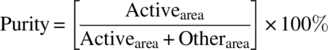
where Otherarea refers to the peak areas of all the other peaks in the chromatogram.
Thus any impurity is assumed to have the same response factor as that of the main component. The reason area% purity is reported is one of timing. In early development of a new chemical entity, there are usually no standards. As area% purity is something that can be reported from the first injection, a meaningful metric can be generated without a lot of work to develop standards. The area% purity values can be used to compare the historical samples with each other to compare differing chemical approaches to the project. Later on in the project, when standards have been made and characterized, percent purity by mass values can also be reported. This percent purity by mass relative to the standard (also referred to as potency) taken with the percent purity by area value is a good indicator of how well the standards are characterized. For the remainder of this chapter, the percent purity by area will be referred to as just purity.
6.2.2 Potency
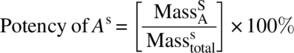

- Superscript S denotes sample.
- Superscript STD denotes standard.
- Subscript A denotes material A.
The term potency in Eq. (6.2) is a bit deceiving at first glance as it appears that when samples are reported at a given percent potency, then this is a percent by mass intrinsic to the test sample. This is not the case. Actually this value is a percent active compared to an external standard as shown in Eq. (6.3) through the use of a proportionality constant called a response factor designated by Rf. This response factor is generated from a reference standard as shown in Eq. (6.4) by taking the ratio of the response, HPLC area in this case, to the mass of the sample. The reference standard is typically a well‐characterized purified sample of the desired material used to calibrate HPLC peak area to mass of the sample. In most cases in the pharmaceutical industry, the reference standard is not commercially available and has to be purified by thorough crystallization or preparative‐scale chromatography.
Response factors can be simplified as the ratio of the output response to the input material and is used in most analytical technique with linear responses such as mid‐IR spectroscopy, mass spectroscopy, or in this case ultraviolet (UV) spectroscopy. After close inspection of Eqs. (6.2)–(6.4), it becomes apparent that the accuracy of the potency value hinges on the quality of the standard used to generate the response factor. As all reported values are relative to the standard, it is possible to have a test result indicating a potency greater than 100%, indicating the sample is more potent than the standard.
Early in development, this standard may be nothing more than the most pure obtained sample to date. The limited characterization of the standard consists of analysis for residual solvents including water as well as residue on ignition testing (ash). Anything that is not ash or solvent is then attributed to the material of interest. So to reiterate, potency refers to the % active component in a given sample relative to an external reference standard for that active component.
TABLE 6.1 Possible Scenarios of Purity and Potency Values
| Purity: |
Potency: |
|
| Purity = potency | Can occur if the response factors of all the UV‐active components including impurities are very similar so that an area% of A is equivalent to a wt %. It also requires that the reference standard for the potency determination be highly accurate | |
| Purity < potency | If we assume the reference standard is accurate, then this situation can arise if the impurity peaks have a higher extinction coefficient and higher absorbance than the desired component A. This translates to artificially high impurity count and lower purity by area% | |
| Purity > potency | If we assume the reference standard is accurate, then purity will exceed potency when there are non‐UV components present that are not being detected by HPLC. This will contribute to lower potency values and higher HPLC area% – for example, if the sample has high salt content (ash). This will look pure by HPLC because the ash is not detected | |
| Potency > 100% | Reference standard likely not well characterized with respect to wt % ash, residual solvent, or impurities | |
For comparing processes with each other based solely on isolated yield and relative potency, a less than fully characterized standard still allows for relative comparison, i.e. 103% potent material is better than 95% potent material. For work that would require a more stringent mass balance, kinetics, or process understanding, the mass balance should be closed by utilizing a combination of complementary analytical techniques such as quantitative H1‐NMR and HPLC.
Two areas where analytical data are most frequently needed by the API process development engineer are data to close the mass balance and data to develop kinetic models. These two utilizations of the data are not independent of each other, as it is necessary to have a reasonable mass balance before attempting to develop a kinetic model. As such it is imperative to have analytical techniques available that can both “see” what needs to be tracked and give values of concentrations that are needed for both the mass balance and the kinetic model.
6.3 METHODS USED AND BACKGROUND
What follows is a brief overview of the most common analytical techniques used and some concepts that need to be kept in mind when attempting to analyze the data generated. A more thorough discussion about each technique can be found elsewhere [1].
All methods of column chromatography rely on the same basic principles. First there is a sample that is made up of a mixture of components. This mixture is loaded onto a column that separates the individual components as they partition between two phases, the mobile and the stationary phases. In liquid chromatography (LC), the partitioning is driven by the polarity of the components and the differing polarity of the mobile phase versus the stationary phase, absorbing and de‐absorbing onto the stationary phase down the length of the column. In gas chromatography (GC), the partitioning is driven by the relative volatility of the components as it alternates between the gas phase and dissolution into the stationary phase. The net effect of any chromatographic system is to separate the components of the sample mixture. It is the detector that is attached to the outlet of the chromatographic system that allows one to see the relative concentrations of each species in the sample. As such, the type of detector used will dictate what is “seen” by the analytical method. Table 6.2 lists the types of detectors available, what type of chromatographic system they are most often paired with, and what they are capable of detecting.
TABLE 6.2 Properties of Most Common Detector Types
Source: From Ref. [2].
| Chromatography Method | Detection of | Sensitivity | Notes | |
| Ultraviolet (UV) | LC | Absorption of UV light by pi─pi bonds, i.e. conjugation | Dependent on ε of the analyte | Variation of ε on the order of 100‐ to 1000‐fold is possible |
| Mass spectrometer (MS) | LC/GC | Charged particles | μM concentrations | Does not detect mass but rather mass to charge m/z ratio |
| Flame ionization detector (FID) | GC | Ionized particles from combustion of organic compounds | ppm–ppb | Signal proportional to number of carbon atoms, i.e. signal proportional to mass not concentration |
| Conductivity | LC | Charged ions by measuring resistance in detection cell | 5 × 10⁻⁹ g/ml | Most often used for ion exchange chromatography |
| Electrochemical | LC | Current generated by oxidation or reduction of sample | Order of magnitude more sensitive then UV | More selective and sensitive then UV, but detector not as rugged as UV |
| Refractive index (RI) | LC | Variations in refractive index | 0.1 × 10⁻⁷ g/ml | Universal detector, poor detection limit, sensitivity to external condition (temperature, dissolved gas, etc.) limit practical use |
| Evaporative light scattering detector (ELSD) | LC | Nonvolatile particles of analyte scattering light | 0.1 × 10⁻⁷ g/ml | Analyte needs to be nonvolatile were mobile phase needs to be volatile |
| Fluorescence | LC | Low ng/ml range | Typically require derivatization with fluorophore reagents |
The underling similarity in all these methods of detection excluding FID is that the resulting signal is proportional to the concentration. The important thing to remember is that for every component of a sample that is being analyzed, there is a proportionality constant that is unique to that compound. So in the example of the UV detector, the most common detector for different LC methods, this proportionality constant is the molar absorptivity ε. The relationship of ε to concentration and absorption is described by Beer–Lambert law shown in Eq. (6.10):
where
- A = absorption, dimensionless
- ε = molar absorptivity, L/mol/cm
- c = concentration, mol/L
- b = detector path length, cm
In the case of mass spectrum (MS) detectors, the proportionality constant is the ionization potential; in electrochemical detection, it is the RedOx potential. Even in the case of non‐chromatographic methods, the idea of proportionality constants should always be remembered. As an example quantitative NMR has relaxation times that can be thought of as proportionality factors. So for every sample analyzed, be it with chromatography or not, the individual components each will have a unique proportionality constant that may or may not be similar to other components in that sample. This is why most detectors are not universal detectors; all species that are chemically different will have different proportionality constants. In many instances if the components are all structurally similar, then their proportionality constants may be very similar as well, but this is not always the case. This is why taking area% values as direct replacements for concentration can lead to erroneous results. At best these area% values can be used to indicate relative abundances, but care around the possibility of different response factors must be taken if area% values are used as replacements for concentration values for calculating mass balances or kinetic profiles. The following example illustrates this point.

FIGURE 6.1 Conversion as calculated by the chemist in the lab by Eq. (13.6) only taking the ratio of starting material and product area% into account.
FIGURE 6.2 Conversion calculated by Eq. (13.6) shown as solid line compared with conversion calculated by Eq. (13.7) shown as solid box. This discrepancy between the two values at the 48 hours time point indicates that the forced mass balance of Eq. (13.6) elevated the product concentration as by not taking into account a possible side reaction of the starting material that did not result in product.
6.3.1 Mechanics of HPLC and UPLC
HPLC and the more recent ultra‐pressure/performance liquid chromatography (UPLC) are considered the standard lab equipment when it comes to understanding what is going on in a synthesis or process. The difference between these two techniques lies in the size of the solid‐phase packing in the columns as well as the pressures that are employed, hence the high/ultra descriptors. For HPLC the solid‐phase packing is between 5 μM–3 μm and 200–400 bar pressure, where UPLC solid phase is below 3 μm in size and pressures above 1000 bar.
A quick aside about the equation that governs the efficacy of both techniques, as well as any other column chromatography, the van Deemter equation is in its simplified version (Eq. 6.14) [3].
where
- H (sometimes shown as HETP) is the variance per unit length, also referred to as height equivalent to a theoretical plate.
- u is the volumetric flow rate.
- A is the term describing the multipaths in the packed bed.
- B is the term describing longitudinal diffusion.
- C is the term describing resistance to mass transfer.
This hyperbolic function relates the variance per unit length to particle size, mass transfer between the stationary and mobile phases, and the linear velocity of the mobile phase. This relationship was the first result from applying rate theory to the chromatography process and was originally developed to describe GC. It has been extended to describe LC as well with modifications to the lumped parameters terms A, B, and C in Eq. (6.14). A typical van Deemter plot is shown in Figure 6.3.
FIGURE 6.3 Characteristic van Deemter plot shape illustrating the presence of an optimum flow rate to maximize column efficiency.
The van Deemter equation is useful in describing the theory and mechanism of the chromatography process, not only for the small analytical chromatography used in analysis but also for large‐scale separations done on large pilot plant and commercial scale. This equation explains why the problem of unresolved peaks cannot be solved by just going to a longer column at the same flow rate. The increased resolving power of more packing in a longer column is lost to the increase of the B term in Eq. (6.14) (increase of eddy and longitudinal diffusion) due to increased time spent on the column. Thus the number of theoretical plates is less for the longer column (when held at the same flow rate) even though it is longer with more packing because the height of the plates, the H term in Eq. (6.14), is larger as well. This is where UPLC comes into its own. By decreasing the packing size and increasing the pressure, the linear velocity is kept high, and the increased resolving power of more packing is not lost to increased diffusion, thus giving higher plate counts for a given time on the column. The net result is increased resolution and throughput for the analyses.
Both methods, HPLC and UPLC, are only a tool for separating individual components from a mixture and feeding them to a detector that will give a response that is proportional to concentration. It is concentration data that are typically the most applicable to the engineer, and their accuracy is of foremost importance.
6.4 THINGS TO WATCH OUT FOR IN LC AND GC
6.4.1 Injections Have Everything in Them Not Just the Desired Reactants
The first thing that must be communicated to the analyst, or kept in mind for those that are acquiring their own data, is to account for what is in the reaction mixture. The most common mistake in LC that everyone makes once and hopefully only once is the toluene mistake. This is what happens when people forget that toluene unlike most organic solvent has both a chromophore and is retained on most LC columns. I cannot tell you how many bright analytical chemists have come running down in a panic telling everyone that there is this major new impurity only to find out that the project has switched to toluene in the process and had not notified the analyst. Worse yet is the chemist that reports that they have excellent in situ yield only to be looking at a nonexistent reaction because they assumed that large peak that was not starting material was product when in reality it was the toluene peak. This can lead to wasted development time chasing a nonexistent reaction.
In GC the major concern is nonvolatiles, i.e. salts. If a lot of reaction mixtures that contain large percentages of salts are injected, then the injector may become plugged, necessitating in cleaning the injector before accurate analysis can resume. What is more complicated is when the product or reactants are salts, i.e. charged species. These will not “fly” on the GC and will require some sort of quench to run on the GC. Most often this is a neutralization of the reaction mixture to quench the charge on the desired compounds so as to facilitate GC analysis.
6.4.2 Unplanned/Planned Modification of Stationary Phase
If running one's own analysis, one must be cognizant of possible changes to the HPLC column due to history. Depending upon the nature of the mobile phase being used, “conditioning” of the column may take place such that the results may not be repeatable, or representative of differing HPLC system. This opens the possibility of analysis that cannot be duplicated, leading to confusion around what results are accurate. A prime example of conditioning of the column is ion‐pairing mobile phase such as sodium dodecyl sulfate, or a weak ion‐pairing agent such as perchloric acid. In the case of ion‐pairing mobile phases, the stationary phase is modified or conditioned over time to be more retentive of polar species such as primary amines due to the stationary phase being modified by the mobile phase containing the ion‐pairing agents. There is a memory effect now for this column that will still maintain the effect even if the mobile phase is switched to a more traditional acidic mobile phase. This has the greatest impact when someone develops a method with such a conditioned column as it will be impossible to replicate these results without this preconditioned column.
The other extreme is when the column is conditioned negatively or destroyed by running samples of reaction mixtures that destroy the resolving power of the stationary phase. This is most often seen with samples from reactions such as hydrogenations that contain metal species that bind to the stationary phase, resulting in reduced resolving power. If a column is suspected of being conditioned either negatively or positivity, then the only option available is to replace the column and see if the previous analysis is replicated. Thus it is always good to periodically run a system suitability test to check analytics with a reference mixture to confirm retention times/peak shapes.
6.4.3 Product Stability/Compatibility with Analysis Method
Stability of the reaction mixture or products to the chromatographic conditions is another major concern that needs to be addressed before a strategy for analyses can be agreed upon. The majority of aqueous mobile phases utilized in UPLC and HPLC are acidic. This regularity of acid mobile phases is due to two major factors. The first factor is that until recently the silicon support for the column mobile phase was not stable to high pH values as silicon is soluble at pH levels above 11. The second factor is that if the mobile phase pH is near the pKa of any of the sample components, then slight variations in the pH of the mobile phase can change the polarity of the components. This change in polarity will then change retention time and order of elution of the components.
Because of these two factors, the majority, near 80% of the mobile phases, is acidic (pH < 1) to both maintain the stability of the mobile phase as well as to prevent any change in the analysis due to pH variations. The idea is to protonate everything and prevent pH gradients from forming on the column that may cause chromatographic artifacts.
This proclivity of mobile phases to be acidic makes stability to acid aqueous conditions one of the main stability concerns. As the amount of sample that will be loaded on the column for each injection is so miniscule, in the order of microliters, the sample gets swamped by the mobile phase. If the sample is not stable to aqueous/acidic conditions, then degradation will be taking place as the sample travels and elutes from the column. The net effect is that the sample that was representative of the reaction at a given time or point in the process is scrambled by the analysis method, rendering the results no longer representative. This is unfortunate if one lab‐scale reaction is lost because of this, and devastating if three weeks of DOE experimentation is rendered useless also because of this; both have happened.
In GC the major issue with stability of the reaction mixture is that of thermal stability. Remembering that the standard injector temperature for GC is 280 °C, this is the temperature that the reaction samples have to “endure” just to get on the column.
If stability is a problem in LC or GC, then quenching the reaction samples (if this improves stability) or some sort of derivatization method may be required.
6.4.4 Derivatization
Derivatization is the process by which a reaction sample is further reacted to form a new compound as part of the sample preparation. This may be done for various reasons such as increasing reactant stability to the analysis method, or modifying the components of a sample to make them detectable such as attaching a chromophore, or to increase volatility for GC analysis [4]. The major issue with derivatization is that this is a second reaction that is in series with the desired reaction. The net effect of this is that if the reaction of interest is to be accurately characterized, then the derivatization reaction needs to be quantitative in reaction completion and at a reaction rate that is orders of magnitude faster than the desired so as to not skew the analysis. For a system that a kinetic model is being developed and derivatization is required, a quench of the reaction should be used before derivatization or a derivatization that also quenches the reaction. This is to ensure that the analysis is representative of the time the sample was taken, not the time the sample was analyzed.
6.5 USE OF MULTIPLE ANALYTICAL TECHNIQUES
Oftentimes when trying to understand a process by developing a mass balance as well as a kinetic model, it is best to start at the beginning. In most cases the beginning is a full characterization of the feedstocks going into the process. It will be very difficult to close the mass balance if one is not aware of what is going into the process. The use of two or more complementary analytical techniques can greatly aid in fully understanding the inputs for a process. The following Case Study 6.1 illustrates this point.
6.6 CONCLUSION
The use of analytical methods to elucidate process parameters be it mass balance or ultimately kinetic information can be full of assumptions. Oftentimes in the pharmaceutical industry, tight timelines prevent the investigation into every assumption. Being aware of the assumptions is the only way that one is ever going to be able to test the ones that will have the biggest impact on the data. The key to understanding what assumptions are being made is being aware of what each analytical method is looking for and what it is proportional to and understanding the complimentary test methods that can give a clearer picture of the problem.
REFERENCES
- 1. Meloan, C. (1999). Chemical Separations Principles, Techniques, and Experiments. New York: Wiley.
- 2. Snyder, L.R., Kirkland, J.J., and Glajch, J.L. (1997). Practical HPLC Method Development, 2e. New York: Wiley.
- 3. Skoog, D.A., Holler, F.J., and Nieman, T.A. (1998). Principles of Instrumental Analysis, 5e. Orlando: Harcourt Brace & Co.
- 4. Little, J.L. (1999). Artifacts in trimethylsilyl derivatization reactions and ways to avoid them. Journal of Chromatography A 844: 1–22.