40.2.1 Absorption Theory: Beer–Lambert Law

The absorption from a single species i at wavelength λ, A_λ, is proportional to the product of the absorption coefficient at the wavelength λ, α_λ; the path length, L; and the species concentration, C_i:

(40.1)

In theory the concentration of species i could be determined by collecting spectra and using a single wavelength for the calibration. Assuming that compound i absorbs at multiple wavelengths, these absorptions could be combined to develop a multiple regression fitting of C_i with n wavelengths:

(40.2)

(40.3)

(40.4)

(40.5)

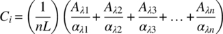
Combining terms for the constants to generate coefficients b₁, b₂, b₃, …, b_n,

(40.6)

Then a multiple regression equation for C_i results:

(40.7)

Figure 40.1 shows data from laboratory experiments for disappearance of a starting material (SM) (reactant) in a batch reactor from grab samples taken as a function of reaction time. The FTIR absorption noted for the SM was clear of overlap from other species in the system at a wavelength of 1397.32 cm⁻¹. Hence, simple linear regression of the first derivatives at 1397.32 cm⁻¹ was tested as an option to build a calibration model for the residual SM. The model, built using 72 data points collected in four experiments, yielded unsatisfactory predictions for the residual SM using spectra collected in a fifth experiment (Figure 40.1, hollow squares). Next, a multiple regression model was created to enable fitting the residual SM concentration (as determined by off‐line HPLC analysis of grab samples, PA%) to the mid‐IR absorbances collected in four of the experiments. The model was built using absorbances at four wave numbers and included three statistically significant two‐factor interactions. The model was then applied to the absorbance data from the fifth batch (hollow squares) to predict the SM concentration profile and compared to the corresponding HPLC data (Figure 40.2).

The data suggest that the fit of the model to the calibration data from the four trials was excellent, but the model was not capable of accurately predicting the behavior of the fifth batch, particularly in the lower PA% region, which is the region of main interest to determine reaction completion in manufacturing batches. These examples from a complex reaction system illustrate cases where simple calibration models are unsatisfactory. Calibrations using a single wavelength, or multiple regression of absorbances from a few wavelengths, can be appropriate in some cases. For example, simple models may be suitable for analysis of solutions of high purity drug prepared for solubility determination.

In most systems of interest in pharmaceutical development, other species (reactants, solvents, related‐substance impurities, etc.) may be present that absorb at the same wavelength as the molecule of interest. Hence, we need to consider the contributions from more than one component to the observed absorption, in addition to more than one wavelength:

(40.8)

(40.9)

(40.10)

where

• A_n is the absorbance at the nth wavelength.
• α_ni is the absorbance coefficient at the nth wavelength for the ith component.
• L is the path length.
• C_i is the concentration of the ith component.
• i is the number of components.

This framework now has the absorbance at a given wavelength properly determined by the sum of the absorbances at that wavelength for each of the i components. The equation may be expressed in a modified form, taking b as the product of the absorption coefficient and the path length, wherein it becomes

(40.11)

This expression further simplifies to the matrix equation:

(40.12)

Here A is a single‐column absorbance matrix with n rows, (n × 1). B is a matrix of constants with n rows and i columns, and C is a single‐column concentration matrix with i rows, (i × 1). Hence, A(n × 1) = B(n × i) × C(i × 1). The B matrix is essentially a matrix of the absorbances produced at the n wavelengths with each of the i components at unit concentration.

It is a simple matter to extend the situation to the collection of spectra from more than one sample, each spectrum being generated from the unique concentrations of C₁, C₂, C₃, …, C_i in the sample.

Let A_ns be the absorbance at the nth wavelength for sample s, b_ni be the absorbance coefficient for at the nth wavelength times the path length for the ith component, and C_is be the concentration of the ith component in the sth sample, where there are n total components or chemical species. Now again we have the matrix equation, but now the A matrix will have a column for each spectrum, and the C matrix will have a column of concentration values for each sample. The matrix equation above holds, but now A is a s column absorbance matrix with n rows, C is s column concentration matrix with i rows, and B is a matrix of constants with n rows and i columns. Hence, in the matrix equation, A(n × s) = B(n × i) × C(i × s).

This forms the basis for calibration of spectroscopic data by the method of classical least squares (CLS). CLS involves the application of multiple linear regression to the Beer–Lambert equation of spectroscopy. A serious drawback of this approach is that the mathematics involved requires there be as many samples as there are wavelengths used in the calibration, and there may be hundreds of wavelengths being measured. To overcome this drawback, chemometricians rely on factor spaces and factor‐based techniques, chiefly principal component analysis (PCA), PCR, and PLS.

40.2.2 Principal Component Analysis

PCA is an orthogonal mathematical transformation to convert a set of observations that may be correlated into a smaller set of linearly uncorrelated variables termed the principal components, which are eigenvectors. In doing so, the dimensionality of the data set is reduced. For example, an IR spectrum with absorbance values measured at several hundred wave numbers may be reduced to considerably fewer, perhaps a handful of, principal components after PCA. PCA itself does not perform a regression; rather it operates on a set of data. Hence, p variables will end up with a set of p principal components [4].

The first principal component, PC1, is selected by finding a vector describing the maximum variation in the data set. To find the second principal component, PC2, a vector orthogonal to the first is identified that explains the greatest amount of the remaining variation in the data set. Additional principal components are found in this manner until the variation in the data set is explained to within the expected variation due to random error or noise. The determination of the appropriate numbers of principal components to include can be done by a variety of numerical methods. This is essential to avoid overfitting the data and creating inaccurate predictions by including too many factors that describe random error and noise. PCA by itself does not directly yield quantitative values for prediction of concentrations in samples, but is extremely useful to compare data collected under different processing conditions, such as monitoring reactions or crystallizations performed at different temperatures, reagent concentrations, etc.

To help visualize how principal components work, consider a two‐component system, a mixture of A and B. A solution of component A is prepared at exactly unit concentration (C = 1). Data are collected using a hypothetical spectrometer for which the spectra are assumed to be error‐free, and the absorbances measured at three wavelengths, λ₁, λ₂, and λ₃. Similarly, a solution of component B is prepared at exactly unit concentration, and the absorbances are measured at the same three wavelengths, λ₁, λ₂, and λ₃. The results are as shown in Table 40.1. A solution with no A or B is analyzed, and it shows zero absorbance at the three wavelengths. Next, additional solutions of A and B at various concentrations, including mixtures, are prepared. From Beer's law, for a solution of A prepared at twice the unit concentration, the absorbances will exactly double. Similarly, the absorbances from a mixture of A and B can be calculated by summing the product of their concentrations and the unit absorbances at each wavelength. The results for a series of these hypothetical noise and error‐free measurements on these samples are also shown in Table 40.1.

Conc. of A	Conc. of B
0	0	0	0	0
1	0	1	0.5	0.25
2	0	2	1	0.5
3	0	3	1.5	0.75
0	1	0.25	0.5	1
0	2	0.5	1	2
0	3	0.75	1.5	3
1	1	1.25	1	1.25
1	2	1.5	1.5	2.25
1	3	1.75	2	3.25
1	4	2	2.5	4.25
1	5	2.25	3	5.25
1	6	2.5	3.5	6.25
1	7	2.75	4	7.25
2	1	2.25	1.5	1.5
2	2	2.5	2	2.5
2	3	2.75	2.5	3.5
2	4	3	3	4.5
2	5	3.25	3.5	5.5
2	6	3.5	4	6.5
2	7	3.75	4.5	7.5
3	1	3.25	2	1.75
3	2	3.5	2.5	2.75
3	3	3.75	3	3.75
3	4	4	3.5	4.75
3	5	4.25	4	5.75
3	6	4.5	4.5	6.75
3	7	4.75	5	7.75
4	1	4.25	2.5	2
4	2	4.5	3	3
4	3	4.75	3.5	4
4	4	5	4	5
4	5	5.25	4.5	6
4	6	5.5	5	7
4	7	5.75	5.5	8
5	1	5.25	3	2.25
5	2	5.5	3.5	3.25
5	3	5.75	4	4.25
5	4	6	4.5	5.25
5	5	6.25	5	6.25
5	6	6.5	5.5	7.25
5	7	6.75	6	8.25
6	1	6.25	3.5	2.5
6	2	6.5	4	3.5
6	3	6.75	4.5	4.5
6	4	7	5	5.5
6	5	7.25	5.5	6.5
6	6	7.5	6	7.5
6	7	7.75	6.5	8.5

Next, we can visualize the spectra in three‐dimensional space by plotting the absorbance of the first wavelength along one axis, the absorbance of the second wavelength along a second axis, and the absorbance of the third wavelength along the third axis. Figure 40.3 shows the plot for the data in Table 40.1.

Note that the spectra, although measured at three wavelengths, lie in a two‐dimensional plane. Regardless of how many wavelengths are used in the measurements, even cases where several hundred wavelengths are used, the data for two components will lie in a two‐dimensional plane. The principal components are then found by finding the eigenvector in the direction of maximum variation of the data set and then a second eigenvector orthogonal to the first in a direction that accounts for the most of the remaining variation in the data set. The first principal component must lie in the plane of the data points to span the maximum possible variation of the data. Similarly, the second principal component will be orthogonal to the first but also lies in the plane of the data set. The principal components for this system are also shown in Figure 40.4. Note that the first principal component explains greater than 87% of the variation in the data set and the second explains a little less than 13%.

It is apparent that we could define a pair of axes in this plane that form a new coordinate system to plot the data and then describe each spectrum on the basis of the distance from the two new axes. This would reduce the dimensionality from 3 to 2. Similarly, had we used three chemical species, A, B, and C, and made similar measurements, the PCA would reduce the dimensionality to a data set described by three new axes.

For each of the data points, the distance of the data point from the PC1 or PC2 vector, often described as the projection of the data point onto the PC1 or PC2 vector, is called a score value. Scores are computed for each data point with respect to PC1 and then again for each data point with respect to a different principal component, typically PC2. Thus a score plot is created, PC1 versus PC2, which allows visualization of how different samples are related to one another. The eigenvalue of the eigenvector is the sum of squares of the projections of the data onto the eigenvector, and the projections are of course the distance along the vector of each data point. Principal component plots, termed loading plots, allow identification of how different variables are related to each other. Working with scaled variables is preferred, since the PCs and scores then become dimensionless variables.

Most commercial software packages output the eigenvalues of the principal component, as well as the relative amount of the variation in the data that is explained by each principal component, enabling interpretation as to the number of vectors needed to reduce the dimensionality of the data set.

40.2.3 Principal Component Regression (PCR)

For spectra collected on a set of samples of known concentration, the principal components of both the absorbances, X, and the known concentrations, Y_n, can be calculated. For the set of observations, the matrix of regression coefficients, B, is computed:

(40.13)

This is termed building a calibration model. As additional spectra on samples of unknown concentration are collected in the future, it is possible to estimate the concentration of the unknowns, Y_u, from the calibration model and the measured absorbance, X_u:

(40.14)

40.2.4 Partial Least Squares

PLS is an extension of PCR where again both the X and Y data are considered. However, the PLS equation or calibration is based on decomposing both the X and Y data into a set of scores and loadings, similar to PCR, but with one significant difference: the scores for both the X and Y data are not selected based solely on the direction of maximum variation, but instead are selected in order to maximize the correlation between the scores for both the X and Y variables. The result is termed a set of latent vectors, or basis vectors, or sometimes simply factors. The selection of the appropriate number of factors is important to properly fit the model, and the software packages have built‐in capability to recommend the number of factors to keep based on the predicted residual error sum of squares (PRESS residuals). Most commercial software packages [5] come with the ability to do PCA, PCR, and PLS.

PLS decomposition of X and Y into scores and loadings [5, 6] is given as

(40.15)

(40.16)

T and U are the score matrices for X and Y and P and Q are the loading matrices. PLS does not calculate the scores independently, but rather it seeks optimal congruence of the u and t vectors by using the u vector as the starting point for calculating the t vectors. This self‐consistent approach allows for a set of scores and loadings that represent the variation in the Y data set. Therefore, the scores and loadings are much better than PCR scores [4, 5] and loadings for quantitative prediction; hence PLS regression is the preferred technique for building calibration models and unknown prediction. The algorithm proceeds by mean centering the data and then finding the first loading spectrum and first component scores. The prediction of a PLS method is summarized in the regression vector or coefficient, B. The predictions are related to the X sample data by equation (Y = BX).

40.2.5 Data Preprocessing

It is important to note that while chemometric techniques may be applied to raw absorbance values, this is not usually the case. Before performing the various multivariate calibration and prediction techniques, some form of data transformation or preprocessing, while not mandatory, is nearly always warranted. There can be bias in the estimates if the predictors and the response variables are significantly different in magnitude, resulting in unequal leverage. Hence, each variable may be scaled by its mean and standard deviation to place the predictors and responses on more equal footing. Scaling the data at each wavelength as well as scaling of the response data used to derive the calibration is common. In fact, mean centering and scaling is so commonplace that some investigators take it for granted and do not report that they performed it prior to the analysis.

Derivative processing is common with mid‐IR and NIR spectra. Taking the first derivative of the spectra corrects for baseline shift during the data acquisition. Taking the second derivative of the spectra corrects for baseline drift. There are several methods for calculation of the spectral derivatives, with the most common being the method of Savitzky–Golay [7]. Examples of the raw absorbance spectrum and the resulting first derivatives of the spectra are shown in Figures 40.5 and 40.6.

Depending on the sample type, particulate containing slurries and solutions may show light scattering effects with mid‐IR or NIR, and Raman spectra may exhibit background scattering. Hence, another technique applied to the spectra depending on the amount of diffuse reflectance is the multiplicative scattering correction (MSC). The pretreatments can be applied to the spectra or to the response data (y‐data).

REFERENCES

- 1. ICH (2012). International Conference on Harmonisation of Technical Requirements for Registration of Pharmaceuticals for Human Use, Development and Manufacture of Drug Substances (Chemical Entities and Biotechnological/Biological Entities) Q11, Step 4, 1 May 2012.
- 2. U.S. Food and Drug Administration (2004). Guidance for Industry Process Analytical Technology. Rockville, MD: U.S. Food and Drug Administration.
- 3. Ehly, M. and Gemperline, P.J. (2007). Analytica Chimica Acta 595: 80–88.
- 4. Kramer, R. (1998). Chemometric Techniques for Quantitative Analysis. Boca Raton, FL: CRC Press, Taylor & Francis.
- 5. Esbensen, K. (2002). Multivariate Data Analysis – In Practice. Oslo, Norway: CAMO Process AS.
- 6. Chiang, L.H., Russell, E.L., and Braatz, R.D. (2001). Fault Detection and Diagnosis. London: Springer.
- 7. Savitzky, A. and Golay, M.H.E. (1962). Analytical Chemistry 36: 1627–1639.
- 8. Martens, H. and Naes, T. (1989). Multivariate Calibration. Chicester: Wiley.