
18
APPLICATIONS OF THERMODYNAMICS TOWARD PHARMACEUTICAL PROBLEM SOLVING
Ahmad Y. Sheikh, Alessandra Mattei, and Raimundo Ho
Solid State Chemistry, AbbVie Inc., North Chicago, IL, USA
Moiz Diwan
Process Research and Development, AbbVie Inc., North Chicago, IL, USA
Thomas Borchardt and Gerald Danzer
Drug Product Development, AbbVie Inc., North Chicago, IL, USA
Nadine Ding and Xinmin (Sam) Xu
Abbott Vascular, Santa Clara, CA, USA
18.1 INTRODUCTION
Interplay of thermodynamics and kinetics underpins many aspects of pharmaceutical development. Understanding of the underlying thermodynamics helps conceive, develop, and control a range of processes and the resulting properties/quality attributes. Quality and regulatory considerations also require thorough understanding and robust control of the processes to ensure patient safety. An obvious application of thermodynamics within the context of chemistry, manufacturing, and control (CMC) development relates to the importance of crystal form in solid dosage development. Polymorphism is prevalent for molecular crystals [1, 2], and a recent detailed study showed that well over a third of all pharmaceutical compounds exhibit polymorphism [3]. Polymorphism affects a range of physical properties including melting point, intrinsic solubility, dissolution rate, and stability. These differences are related to thermodynamics and in particular free energy differences often caused by differences in molecular packing configurations. The utility of co‐crystals to modulate biopharmaceutical properties and processability [4–7] also stems from the underlying differences in free energies. Additionally, interactions between components in common multicomponent/multiphase pharmaceutical systems are governed by thermodynamics of mixing.
In this chapter, five distinct case studies are presented to demonstrate a range of approaches to establish and apply foundational thermodynamics in the design and control of a variety of different pharmaceutical processes. The case studies cover (i) desolvation behavior of a polymorphic system, (ii) solid form control during crystallization, (iii) scalable solution crystallization of co‐crystals, (iv) coating process for drug‐eluting bioresorbable vascular scaffold (BVS), and (v) polymer–plasticizer mixing performance in the presence of water.
While the most consequential assumptions inherent in various thermodynamic models are highlighted, a detailed discussion on the actual mathematical constructs is outside of the scope of this chapter.
18.2 DESOLVATION OF PARECOXIB SODIUM
18.2.1 Introduction
Parecoxib sodium is a water‐soluble prodrug belonging to COX‐2 class of drugs. It is administered intravenously [8] and marketed in Europe as Dynastat for short‐term perioperative pain control. The chemical structure is shown in Figure 18.1. Polymorphism studies conducted at Pharmacia Corp. during development in the early 2000s identified three anhydrous (Forms I (A), II (B), and III (E)) and various solvated and hydrated forms [9]. The development of a more soluble (metastable) form (preferably mostly Form I) was desirable from a manufacturing perspective for the IV formulation. None of known anhydrous forms at the time could be isolated directly from the crystallization process and had to be made by desolvation of solvates. Form conversions in the drying process represented significant challenge for robust design, scale‐up, and technology transfer of the API manufacturing process.

FIGURE 18.1 Chemical structure of parecoxib sodium.
18.2.2 Semiquantitative Phase Diagrams
Free energy–temperature and composition–temperature diagrams were considered necessary to understand crystal form landscape and desolvation pathways for parecoxib sodium. For a system comprising “n” solvent‐free forms, “2n” properties need to be measured or determined to construct a sufficiently detailed free energy–temperature diagram [10]. These properties can include but are not limited to melting temperature, heat of fusion, heat of solution [11], solubility, and intrinsic dissolution rate [12].
Thermal data was collected on the nonsolvated forms using Mettler Toledo differential scanning calorimetry (DSC). Form I displayed a single melting endotherm with an onset at about 273.1 °C (ΔHt = 23.8 kJ/mol). Form II displayed an endotherm with an onset at about 195.9 °C (ΔHt = 20.71 kJ/mol) representing transition to Form I, followed by a sharp melting endotherm for Form I at 273.7 °C. Form III displayed a broad endotherm with an onset at about 206.6 °C (ΔHt = 18.35 kJ/mol) representing transition to Form I, followed by a sharp melting endotherm for Form I at 273.2 °C. Qualitative thermal data for the three forms is shown in Figure 18.2.
FIGURE 18.2 Qualitative DSC data for Forms I (a), II (b), and III (c).
The transitions for Forms II and III to Form I prior to melting were verified by hot‐stage microscopy.
Based on the heat of transition rule [13], both Forms II and III can be considered enantiotropically related to Form I. Since, melting and recrystallization events were not sufficiently resolved; calculation of the transition temperature using the standard DSC [14] data was not possible. Method of eutectic melting [15] was therefore employed. It allows modulation of melting points by using reference compounds at eutectic compositions to help isolate melting and crystallization events and accurately determine heat of fusion data. Eutectic compositions and corresponding heat of fusion data can then be used to derive the free energy differences between crystal forms using Eq. (18.1):
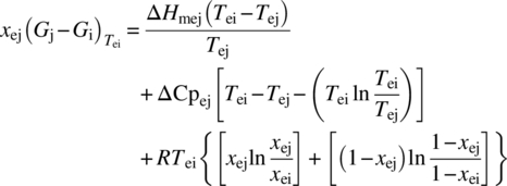
wherein
- xej and xei are the mole fraction of crystal forms j and i, respectively, in the eutectic.
- (Gj − Gi) is the free energy difference between crystal forms i and j at Tei.
- ΔHmej is the enthalpy of eutectic melting of crystal forms j.
- Tei and Tej are the temperatures of eutectic melting of crystal forms i and j, respectively.
- ΔCpej is the heat capacity change across the eutectic melt.
- R is the ideal gas constant.
Plots of (Gj − Gi) vs. T and (Gj − Gi)/T vs. 1/T can then be used to determine two thermodynamic parameters (ΔH and ΔS) essential for determining the transition temperatures (Tt) using Eq. (18.2):
Phenacetin, benzanilide, and salophen were used as the reference compounds to ensure that a broad range of eutectic melting temperatures could be achieved for each of the three anhydrous forms. Physical mixtures comprising varying mole fractions of anhydrous form and reference compounds were prepared, and DSC data was collected. Compositions that led to detection of a single melting endotherm were recorded as eutectic compositions. Thermodynamic properties obtained at eutectic compositions for Forms I, II, and III with each reference compound are given in Table 18.1.
TABLE 18.1 Eutectic Melting Data for Forms I, II and III
| Crystal Form | Form I | Form II | Form III |
| Tm (°C) | 274–276 | Phase conversion | Phase conversion |
| RC = phenacetin | |||
| Xe | 0.25 | 0.25 | 0.25 |
| Te (°C) (mean) | 118.2 | 124.7 | 124.7 |
| ΔHme (kJ /mol) | 24.64 | 25.99 | 27.08 |
| RC = benzanilide | |||
| Xe | 0.17 | 0.18 | 0.18 |
| Te (°C) (mean) | 155.6 | 156.6 | 156.2 |
| ΔHme (kJ/mol) | 28.32 | 31.95 | 31.42 |
| RC = salophen | |||
| Xe | 0.42 | 0.42 | 0.42 |
| Te (°C) (mean) | 171.7 | 170.1 | 170.1 |
| ΔHme (kJ/mol) | 25.82 | 36.83 | 34.62 |
Xe is the eutectic composition on molar basis, Te is eutectic melting point, ΔHme is enthalpy of fusion for the eutectic melt, and Tm is the melting point of parecoxib sodium crystal forms.
Plots of ΔG vs. T and ΔG/T vs. 1/T were used (not shown here) to determine enthalpic and entropic differences between pairs of parecoxib forms, and key thermodynamic parameters are shown in Table 18.2.
TABLE 18.2 Thermodynamic Parameters for Interconversion of Forms
| Form/Transition | Thermodynamic Parameters | ||
| ΔH (kJ/mol) | ΔS (J /[K mol]) | Transition Temperature (°C) | |
| II to I | 16.63 | 38.1 | 163.3 |
| III to I | 17.15 | 39.2 | 163.9 |
The data confirmed an enantiotropic relationship between Forms I and either II or III. Forms II and III were found to be very close in energy, whereas Form I was found to be the highest energy form. The rank order of stability correlated with true density data as measured by helium pycnometry (Form II, 1.46 g/cm3; Form III, 1.42 g/cm3; Form I, 1.34 g/cm3). Similar transition temperatures for Form III/Form I (163.9 °C) and Form II/Form I (163.3 °C) were obtained due to the narrow energy difference between Forms II and III. In fact, the similarity of free energies of Forms II and III makes it difficult to conclusively ascertain the thermodynamically most stable form at ambient temperature. The data were used to construct a semiquantitative G‐T diagram shown in Figure 18.3.
FIGURE 18.3 Semiquantitative G‐T diagram for three anhydrous forms of parecoxib sodium (temperatures in K).
While the G‐T diagram is highly informative in understanding the phase relationships and difficulty of thermodynamically controlling Form II or III, it does not help understand the desolvation behavior of Form IV (ethanol solvate) that was isolated from the crystallization process. Desolvation or decomposition of a crystalline solvate can happen in two distinct environments: under constant composition or steady loss of solvent. For the latter, kinetics of conversion can be key determinant of the outcome, whereas for the former thermodynamics also plays an important role. To understand the thermodynamics of desolvation, experiments need to be conducted to understand the melting behavior of the solvate and determine if it exhibits eutectic or peritectic melting. Eutectic melting occurs when the two components of the solvate melt into each other and remain liquid with no recrystallization. Peritectic melting occurs when a solvate becomes unstable and phase converts in the presence of either saturated headspace or in a solution that has solvent activity of one for solvent of solvation. Phase conversions just above the peritectic temperature tend to be fast, and the resulting solids are usually solvent‐free and most stable at that temperature. Carefully executed sealed pan and open pan DSC and sealed and unsealed hot‐stage microscopy (with appropriate mineral oils) [16] can be used to determine the melting behavior of solvates. Peritectic melting behavior is detected in the DSC by delayed “melting/desolvation” endotherm, immediately followed by a crystallization exotherm and eventual melting endotherm of the anhydrous form. The crystallization exotherm can be sharp or broad depending on scan rate and ability to hold the solvent vapors in the DSC pan. Verification of peritectic melting behavior can be performed by comparing DSC thermal events under unsealed conditions. In this case, earlier onset of desolvation followed by very slow conversion to the desolvated phase or kinetically favored anhydrous phase is often observed.
When such experiments were conducted under sealed conditions with Form IV of parecoxib, peritectic melting to Form III was observed. The peritectic melting point was determined to be approximately 72 °C. Analogous experiments under unsealed conditions resulted in either Form I or II depending on the heating rates and starting solvent content of the wet Form IV. Solid form was confirmed by opening DSC pan after the desolvation event and analyzing the solids by powder X‐ray diffraction.
Melting data on the anhydrous forms, transition temperatures (between anhydrous forms), and peritectic melting point were used to construct a semiquantitative composition–temperature or x‐T diagram (Figure 18.4). It is worth emphasizing that the horizontal axis is exaggerated at both ends of the composition range to clearly illustrate the key features of the system. It is also noteworthy that the left‐hand side of the diagram is purely conceptual and no efforts were made to experimentally determine eutectic composition through solubility measurements.
FIGURE 18.4 Semiquantitative x‐T diagram for the ethanol solvate and three anhydrous forms of parecoxib sodium.
The x‐T phase diagram helps visualize two distinct drying/desolvation pathways (ABC and ADE), which can lead to different polymorphic outcomes. In pathway ABC, the solvent content of solids is at or above mole fraction corresponding to the composition of Form IV solvate when drying temperature approaches/exceeds the peritectic melting point. As a consequence Form IV readily converts to Form III. In pathway ADE on the other hand, most of the solvent is removed below the peritectic melting point, and as a consequence saturation conditions with respect to the solvent are not achieved when the drying temperature approaches/exceeds the peritectic melting point. This results in relatively slow conversion of partially desolvated Form IV to either Form I or II. Kinetics of drying/desolvation play a leading role in the outcome of ADE pathway.
18.2.3 Implications for Process Design and Control
As previously mentioned during development for the IV formulation of parecoxib sodium, Form I or II was more desirable than Form III. Drying process design and scale‐up efforts were therefore focused on efficient removal of the solvent from wet cake below 72 °C. Appropriate washing solvents, heating ramps, mixing protocols, and hold times were established. Only when the established low levels of residual solvents had been achieved was the drying temperature increased to 80 °C to complete form conversion and fully dry the cake. Flexibility was also built into the control strategy with respect to solid‐phase purity of Form I. The process and control strategy was successfully filed with global regulatory authorities and implemented at the commercial manufacturing site.
18.3 SOLID FORM CONTROL OF PARITAPREVIR
18.3.1 Introduction
Paritaprevir is a protease inhibitor [17] that has been developed as part of treatment for hepatitis C virus (HCV). A regimen of three direct‐acting antiviral drugs, with the NS5A inhibitor ombitasvir, and the non‐nucleoside polymerase inhibitor dasabuvir, is marketed in the United States as Viekira. Due to very low solubility of paritaprevir, hot melt extrusion technology [18] is used to manufacture the enabling formulation for drug product.
In the extrusion process, the drug substance is converted from a crystalline solid form to an amorphous state and dissolved in a polymer/surfactant matrix to form an amorphous solid dispersion (ASD) [19]. For HME formulations, low melting crystalline anhydrous forms or hydrates with low dehydration temperatures are preferred to facilitate conversion to the ASD at relatively low temperatures (<200 °C). Given the complexity and structural flexibility of the paritaprevir molecule (see Figure 18.5), numerous crystalline solid forms were discovered during development [20]. Many isomorphic forms (with varying chemical compositions [water or solvents]) were also identified. Class I [21] (or Form II) structures were found to be most suitable for HME formulation. This class represented variable stoichiometry hydrates with similar crystallographic parameters that dehydrated to an amorphous state below a relatively low temperature of 140 °C. Form I, a crystallographically distinct structure, was the most stable under ambient temperature and did not loose crystallinity until 200 °C. Solid‐state conversions between Form I and Form II were, however not observed under ICH stability conditions.
FIGURE 18.5 Chemical structure of paritaprevir.
18.3.2 Solvent Selection and Phase Stability
While Form II had ideal solid‐state properties for downstream processing, slurry competition studies had established that it was only thermodynamically stable at very high water activities (>0.8). For a molecule with very poor aqueous solubility, this presented a very significant challenge for solvent selection and conceptual design of the crystallization process. Extensive solvent screening was conducted to study various combinations of binary and ternary solvents mixtures for solubility, phase purity, and purification potential. Based on these experiments, a solvent system comprising water, isopropanol, and isopropyl acetate was selected. In this ternary solvent system, much of the solubility for the API is attributed to isopropyl acetate. Water content helps regulate water activity and acts as primary antisolvent, whereas isopropanol acts as secondary antisolvent and more importantly as the bridging solvent between water and isopropyl acetate. The fact that an isopropyl acetate solvate and mixed isopropanol water solvate hydrate (Form III) also exist as stable solid form in the ternary solvent system necessitated the construction of sufficiently detailed and robust ternary phase diagram (TPD) for paritaprevir.
18.3.3 Ternary Phase Diagram
Experiments for the construction of four‐component (paritaprevir, water, isopropanol, isopropyl acetate) TPD at 25 and 60 °C was divided into three segments. First the immiscibility boundary for water, isopropanol, and isopropyl acetate was experimentally determined using manufacturing grade solvents. The effect of paritaprevir on the immiscibility boundary was then established. Finally, relative stability of process relevant solid forms was determined for the relevant domains of the solvent space. Immiscibility data from the literature [22] was used to define nine unique experiments in the biphasic space. Details of the overall solvent compositions can be found in Table 18.3. Each experiment was allowed to phase separate in a separation funnel for one hour, before the layers were separated. The composition of the layers was determined through gas chromatography for isopropanol and isopropyl acetate and Karl Fischer titration for water. Mass fraction of each phase was also recorded.
TABLE 18.3 Solvent Ratios for Immiscibility Boundary Determination
| Experiment | Water (g) | IPA (g) | IPAc (g) |
| 1 | 15.0 | 3.0 | 12.0 |
| 2 | 10.5 | 9.0 | 9.0 |
| 3 | 15.0 | 4.8 | 9.7 |
| 4 | 5.0 | 5.0 | 9.0 |
| 5 | 10.0 | 4.0 | 2.0 |
| 6 | 10.0 | 4.0 | 6.0 |
| 7 | 4.0 | 5.0 | 7.0 |
| 8 | 5.0 | 0.0 | 5.0 |
| 9 | 3.0 | 4.0 | 13.0 |
Nine additional experiments were performed to assess impact of paritaprevir on the immiscibility boundary. The amount of added paritaprevir was established based on solubility estimates. Overall compositions for the experiments are captured in Table 18.4. Concentration of paritaprevir was determined using high pressure liquid chromatography. In the experiments where crystallization was observed in any layer, the mixture was heated to 45 °C to dissolve solids before measuring concentration.
TABLE 18.4 Solvent Ratios for Immiscibility Boundary Determination with Paritaprevir
| Experiment | Water (g) | IPA (g) | Total IPAc (g) | Paritaprevir (g) |
| 1 | 15.0 | 3.0 | 12.0 | 0.6 |
| 2 | 10.5 | 9.0 | 9.0 | 0.6 |
| 3 | 15.0 | 4.8 | 9.7 | 0.6 |
| 4 | 5.0 | 5.0 | 9.0 | 0.4 |
| 5 | 10.0 | 4.0 | 2.0 | 0.3 |
| 6 | 10.0 | 4.0 | 6.0 | 0.4 |
| 7 | 4.0 | 5.0 | 7.0 | 0.3 |
| 8 | 5.0 | 0.0 | 5.0 | 0.2 |
| 9 | 3.0 | 4.0 | 13.0 | 0.4 |
The effect of paritaprevir on immiscibility curve at 25 °C is shown in Figure 18.6. The TPD (weight fraction basis) suggests that while the presence of API near saturation levels does not significantly affect immiscibility boundary, the phase separation behavior is nonetheless slightly accentuated by the presence of API. The impact of paritaprevir at 60 °C (data not included) was very similar to 25 °C, most likely due to the lack significant differences in solubility with temperature in the selected solvent compositions. The experimental data without the API collected here with pharmaceutical production grade solvents also show slightly higher degree of immiscibility compared with the literature data [17]. It is, however, difficult to discern if the differences are due to analytical techniques or the subtle differences in actual solvents. Slight quantities of water in isopropyl acetate can, for instance, have significant effect on phase compositions.

FIGURE 18.6 Impact of paritaprevir on immiscibility boundary.
Finally solid‐phase stability was determined via slurry competition experiments in the key domains of ternary solvent space. Physical mixtures of Form II, Form III, isopropyl acetate solvate, and Form I (most stable form under ambient conditions) were used and up to four weeks were afforded for crystal form conversion at 25 and 60 °C. After equilibration, slurries were filtered and solids characterized by powder X‐ray diffraction. Form I was found to be metastable in the entire solvent space, and the isopropyl acetate solvate was only found to be stable in 100% isopropyl acetate. Studies at 60 °C did not result in any changes in the relative stability of the forms. However, the conversion rates were significantly faster at the higher temperature. All the data was used to construct complete phase diagrams. TPD at 25 °C diagram is shown in Figure 18.7 for illustration purposes.

FIGURE 18.7 Complete phase diagram from paritaprevir in crystallization solvent system.
A very cursory assessment of Figure 18.7 shows that much of the solvent space is not suitable for the isolation of Form II under thermodynamic control. Additionally, the narrow domain for II stability is surrounded by regions of either solvent immiscibility or stability for Form III. Both the size and location of Form II domain can therefore present significant challenges for conventional crystallization process design based on, for instance, the use of isopropanol as the antisolvent. In essence regardless of the starting composition for crystallization, the process would need to traverse through regions represented by metastability of Form II or partial miscibility of the solvent system.
18.3.4 Conceptual Design of Crystallization Process
In order to address the challenges captured by the phase diagram, a novel semicontinuous crystallization process was conceived. It afforded maintenance of constant solvent ratio in Form II stability domain throughout the crystallization process.
During the crystallization process, a solution of isopropanol, isopropyl acetate, and water at the final solvent composition was circulated through a high‐speed rotor–stator‐based wet mill. Two separate solutions were prepared: a concentrated solution of paritaprevir in isopropyl acetate and a separate solution with appropriate composition of isopropanol and water. These solutions were added to the circulating solution to initiate and continue crystallization at fixed solvent composition, until the entire product solution had crystallized. Circulation through the high‐speed rotor–stator‐based wet mill also ensured particle size control. Figure 18.8 shows the schematic of the crystallization process. Details of the actual crystallization process can be found in Chapter 27 on Understanding Mixing Effects on Scale‐Up of Crystallizations.
FIGURE 18.8 Crystallization process flow diagram.
Integrity of solid form during the drying process was carefully studied, and appropriate controls were instituted. In the selected drying process, the sequence of “bulk” solvent removal was as follows: IPA, followed by IPAC, and finally water. Throughout most of this sequence, very high relative humidity is automatically maintained in the headspace. During final stages, when most of the solvents are already removed, absolute humidity of no less than 20% was maintained to preserve Form II.
In summary, enabling formulation technology for a poorly soluble API was facilitated through the development of a metastable form under ambient conditions. The metastable form was crystallized under thermodynamic control via a novel semicontinuous API process that ensured very tight control of solvent composition throughout crystallization. Additionally, fundamental understanding of the thermodynamics of solid form across DS and DP manufacture along with the understanding of the physical stability of the metastable form underpinned sound control strategy and robust commercial manufacturing.
18.4 SCALABLE SOLUTION CYRYSTALLIZATION OF CO‐CRYSTALS
18.4.1 Introduction
Co‐crystals are made by a wide variety of techniques including slow solvent evaporation [23], solution crystallization [24], solid‐state grinding (dry grinding and grinding with solvent‐drop addition) [25–27], sublimation and growth from melts [28], and slurry conversions [29]. Slow evaporation and grinding seem to be the most commonly used techniques for isolating co‐crystals. Their prevalence primarily stems from the ability to quickly and simply screen for co‐crystals. Large‐scale production of crystals is, however, usually achieved most robustly through solution (cooling/antisolvent) crystallization [30]. Solution crystallization also offers opportunity for purification and particle size and shape control. Successful outcome of a solution co‐crystallization experiment is predicated on sound understanding of domains of thermodynamic stability in multicomponent solid–liquid‐phase equilibrium diagrams. Building on this essential requirement, we proposed a co‐crystallization process design concept [31], wherein three essential features of the overall approach are (i) rational solvent selection, (ii) demarcation of domains of thermodynamic stability in the multicomponent solid–liquid‐phase equilibrium diagram, and (iii) control of desupersaturation kinetics for desired process performance. Some of these concepts are illustrated in the following case study using carbamazepine–nicotinamide (CBZ–NIC) Form I co‐crystals (see Figure 18.9).

FIGURE 18.9 Crystal structure of CBZ–NIC I highlighting inter‐ring hydrogen bonding interaction for NIC–NIC (bond e) and CBZ–CBZ (bond b) [31].
Source: Reproduced with permission of Royal Society of Chemistry.
18.4.2 Solvent Selection and Ternary Phase Diagram
TPDs are essential to understand thermodynamic stability in multicomponent solid–liquid systems [32, 33]. These diagrams depict the impact of solvent on domains of phase stability and hence provide primary criteria for solvent selection to design the crystallization process. A simple and sufficiently detailed phase diagram can be constructed from solubility data on coformer as a function of API concentration (solid line dividing regions 1 and 6 in Figure 18.10) and API and co‐crystal as a function of coformer concentration (solid lines dividing regions 1 and 2 and 1 and 4, respectively). For a non‐polymorphic single stoichiometry co‐crystal system, three different conceptual TPDs can be drawn to capture the impact of differences in the relative solubility of the API and coformer in different solvents. Figure 18.10 shows scenarios where (a) solubility of the API and coformer are similar, (b) solubility of API is significantly lower than the coformer, and (c) solubility of API is significantly higher than the coformer.

FIGURE 18.10 (a–c) TPDs for single polymorph single composition co‐crystal system. 1, represent liquidus; 2, API and solution; 3, API, co‐crystal, and solution; 4, co‐crystal and solution; 5, coformer, co‐crystal, and solution; 6, coformer and solution.
Very significant practical insights can be gleaned from Figure 18.10. In scenarios (b) and (c), co‐crystal exhibits incongruent dissolution behavior wherein phase change to either coformer or API accompanies a nonstoichiometric solution, whereas congruent dissolution occurs for scenario (a). As a consequence evaporative crystallization, for instance, could only be supported for scenario (a). In scenarios (a) and (c), the concentration of coformer corresponding to its critical activity to stabilize co‐crystal (intersection of regions 1, 4, 5, and 6) is significantly higher than for scenario (b). This could for instance, be detrimental for solution crystallization, where relatively low coformer concentration to achieve co‐crystal stability is more desirable. Higher area of the liquidus region (1) would also have negative consequences for throughput and potentially yield in solution co‐crystallization.
Deeper insights can be gathered by the slopes and lengths of the lines/curve that define the boundaries of liquidus region. The slopes are related to the order of speciation in solution for the API and coformer and provide insights into the consequences of solution‐phase equilibrium. Ability to influence the “length” of the lines by appropriate choice of solvent can have a direct effect on the region of co‐crystal stability. Construction of TPDs as a function of temperature can help identify crystallization trajectories for cooling crystallization that ensure thermodynamic stability throughout the entire process.
As a general principle, the solvent selection criterion is derived from TPD and looks for essential features including (i) high solubility of the coformer compared with the co‐crystal and API and (ii) a very significant difference between the critical concentration of coformer and solubility of coformer. The latter affords the widest window for phase‐pure crystallization of co‐crystals, while the former allows for (i) high throughput (because of the increase in solubility of the API with increasing concentration of the coformer), (ii) large driving force for crystallization of co‐crystals (maximum solubility difference between the API and co‐crystal), and (iii) sink conditions with respect to coformer throughout the crystallization, thereby keeping the concentration of coformer and the solubility of co‐crystal essentially constant during the course of crystallization. Other solvent/solution properties such as deviations from ideal behavior, solvent complexation Kc, solubility product Ksp, and their temperature dependence can be studied to further refine solvent selection.
18.4.3 Co‐crystallization of CBZ–NIC I
18.4.3.1 Solvent Selection
Ethanol, ethyl acetate, and mixtures thereof were used in our study because they provide extremes in solubility of CBZ–NIC I and NIC. Solubility data of NIC and CBZ in ethanol/ethyl acetate mixtures is shown in Figure 18.11. NIC solubility seems to show a very similar trend to nonideal mixing between ethanol and ethyl acetate. The solubility of CBZ on the other hand shows maxima at 0.3 mol fraction ethanol. Using both CBZ and NIC solubility data, it seems that solvent compositions with an ethanol content greater than 0.3 mol fraction (>50% v/v) could best meet the essential elements of the solvent selection criterion (higher differential between NIC and CBZ solubility) described in Section 18.4.2.
FIGURE 18.11 Solubility of CBZ and NIC in ethanol–ethyl acetate solvent system at 25 °C.
The solubility of CBZ–NIC I was measured at 25 °C in four solvent compositions (25, 50, 75, and 100% ethanol in ethyl acetate v/v) as a function of NIC concentration (denoted by [NIC] from hereon). The data captured in Figure 18.12 show that at lower [NIC], solubility of CBZ–NIC I does not follow the general trend of a reduction in solubility with increasing ethyl acetate concentration. Solubility in the low [NIC] region is in fact higher in 75% ethanol than in 100% ethanol. The data also seem to show that a [NIC]critical of greater than 0.97 M required for CBZ–NIC I stability does not vary significantly with solvent composition.

FIGURE 18.12 Solubility of CBZ–NIC I vs. NIC on CBZ basis in ethanol–ethyl acetate solvent system at 25 °C.
The solubility behavior of co‐crystals in solutions of coformers is best described by solubility product (Ksp) and solution complexation (Kc) [24]. Representation of solubility diagrams in these terms is especially useful when comparing the relative merits of different solvent systems. The data shown in Figure 18.12 were transformed and plotted according to Eq. (18.3) to calculate Ksp and Kc values for the four solvent mixture compositions (see Table 18.5):
where [CBT]T and [NIC]T are the total concentrations of two components on molar basis.
TABLE 18.5 Ksp and Kc Values at 25 °C in Ethanol/Ethyl Acetate
| Volume % EtOH | Ksp (M2) | Kc (M−1) | R2 |
| 100 | 0.0096 | 0.521 | 0.99 |
| 75 | 0.0139 | 0.0776 | 0.98 |
| 50 | 0.0105 | 1.7809 | 0.99 |
| 25 | 0.0056 | 6.3428 | 0.95 |
The intercepts of plots used to calculate Kc values in 100 and 75% ethanol are not statistically different from zero, and therefore the values are not expected to be very accurate. Suffice to say that complexation at these two compositions is negligible. Ksp values in the two solvent compositions reflect the greater solubility of CBZ–NIC I in 75% ethanol. As the ethanol content is further reduced from 75%, the expected trend of a reduction in Ksp and increase in Kc is observed. Both the Ksp and Kc values in 100% ethanol compare favorably with the previously reported values [24]. Although very low Ksp value in 25% ethanol helps eliminate this composition from further consideration, the similarity for remaining three compositions does not help in further constraining solvent composition.
Ease of nucleation was used to further refine the solvent selection. Solubility data for CBZ–NIC as a function of temperature and [NIC] in 50, 75, and 100% ethanol was used to determine concentrations of CBZ–NIC I to generate different levels of supersaturation (C/C*) via undercooling. Eight levels of supersaturation were studied to identify onset of co‐crystal nucleation from a clear solution. Table 18.6, summarizing the results, shows that, while the onset supersaturation for 100 and 50% ethanol systems under NIC saturated conditions is similar (ss 1.73 and 1.70, respectively), a significantly higher supersaturation (3.35) is required for nucleation in 75% ethanol.
TABLE 18.6 Onset Supersaturation vs. Solvent Composition and Temperature
| Volume % EtOH | Conc NIC (mg/g) | Temp (oC) | Sol of CBZ–NIC (mg/g) | Ksp (M2) | Onset SS |
| 100 | 95 | 25 | 5.92 | 0.0096 | 1.73 |
| 75 | 93 | 25 | 9.18 | 0.0139 | 3.35 |
| 50 | 62 | 25 | 11.74 | 0.0105 | 1.70 |
| 100 | 47.5 | 45 | 9.49 | 0.0094 | 2.68 |
| 100 | 47.5 | 45 | 30.46 | 0.0521 | 1.48 |
These data along with the high NIC solubility distinguish 100% ethanol as the optimum solvent choice based on both the solution properties and nucleation kinetics. The solubility of CBZ–NIC I in a saturated solution of NIC/EtOH (at 25 °C) was measured as a function of temperature up to 65 °C. A linear van ’t Hoff plot (not shown) was obtained indicating that at the selected [NIC], CBZ–NIC I is stable across the temperature range of interest.
18.4.3.2 Process Design
Based on the understanding of solid–liquid‐phase equilibrium, a conceptual design of solution crystallization was developed. Figure 18.13 shows the block flow diagram.
FIGURE 18.13 Block flow diagram of co‐crystallization process for CBZ–NIC I.
Milled seeds were employed at 2 wt % (CBZ–NIC I basis) to induce nucleation at low supersaturation and to desupersaturate in a more controlled fashion. Post filtration crystals were washed with a 5 mg/g NIC solution in ethyl acetate. This concentration is below the solubility of NIC in ethyl acetate (>8 mg/g) but above the critical NIC concentration for the stability of CBZ–NIC I co‐crystals and therefore allowed for successful removal of the NIC‐rich mother liquor from the wet cake without affecting the stability of CBZ–NIC I during washing. The solids did not have any detectable excess NIC post drying when NIC levels were checked by quantitative HPLC. Yields in excess of 90% were reproducibly obtained for the process.
In summary we have demonstrated a generic approach for designing solution co‐crystallization processes that uses solid–liquid‐phase equilibrium as the foundation of optimum solvent selection and processing trajectories. The methodology has incorporated well‐established techniques and procedures also commonly used in single‐component crystallization to manipulate and control the process for desired performance and product attributes.
18.5 THERMODYNAMICS OF COATING PROCESS DURING THE MANUFACTURE OF DRUG‐ELUTING BIORESORBABLE VASCULAR SCAFFOLD
18.5.1 Introduction
BVSs such as ABSORB™ [34] have the potential to significantly improve treatment of coronary artery disease [35]. Such a combination product consists of a poly(L‐lactide) (PLLA) backbone and a thin coating of 1 : 1 w/w ratio of poly(DL‐lactide) (PDLLA) and everolimus, applied on top of the PLLA backbone. The functional performance of BVS follows three phases: revascularization, restoration, and resorption. In the revascularization phase, the system performs in the same manner as the conventional drug‐eluting stents. Since BVS is designed to disappear over time, in the restoration phase the scaffold starts losing its structural integrity to allow for gradual return of vessel functions. In the resorption phase, the implant is resorbed in a benign fashion, only leaving behind a restored vessel [36, 37].
The overall performance of BVS is influenced by the microstructure of PDLLA/everolimus coating and its relationship to the film coating process. These two aspects affect mechanical property of the coating and in vivo drug release profile. As an extended drug release product with only sub‐milligram quantities of the drug in the device, control of BVS drug release profile is obviously critical for the product performance. Therefore, much scientific, quality and regulatory impetus exists for developing a thorough understanding of the film and processing factors affecting its properties.
The PDLLA/everolimus coating film is typically 1–2 μm in inner diameter and 3–4 μm in outer diameter of PLLA scaffold. It is amorphous in nature and spray‐coated from a 4 wt % solution of 1 : 1 w/w everolimus and PDLLA in acetone [38]. The process involves spraying atomized form of the solution onto the PLLA scaffold backbone, followed by drying to remove the solvent. The resulting film is phase separated in nature, with everolimus‐rich domains dispersed within the PDLLA‐rich continuous phase [39]. Approximately 80% of everolimus within the film is released within 28 days (in vivo), and the elution is fully complete within 120 days [40]. In order to better understand the film‐forming process and properties thereof, an experimental TPD between acetone, everolimus, and PDLLA (solution) was constructed. High‐level details and key findings are summarized in this case study.
18.5.2 Construction of the TPD for Everolimus/Acetone and PDLLA System
Two well‐established aspects of PDLLA/acetone/everolimus include high solubility of both everolimus and PDLLA in acetone (10 wt % each solution in acetone is easily made) and limited miscibility of PDLLA and everolimus. These attributes provide the basic framework to develop a fully descriptive TPD by defining (i) liquidus lines describing change in solubility of PDLLA in acetone as a function of everolimus and vice versa, (ii) solubility/miscibility of PDLLA in everolimus and vice versa, and (iii) immiscibility boundaries between single‐phase and other multiphase regions.
18.5.2.1 Solubility of Everolimus in PDLLA and PDLLA in Everolimus
As a first pass estimate, Flory–Fox [41] equation was used to estimate the solubility/miscibility of PDLLA in everolimus and vice versa. Solubility of PDLLA in amorphous everolimus was estimated to be approximately 8% by weight, whereas the solubility of everolimus in PDLLA was estimated to be approximately 5% by weight. Semiquantitative Raman mapping experiments were conducted to confirm that the estimates are sufficiently accurate. A direct thermal scanning method by Sun et al. [19] was also attempted; however relatively low solubility of the two components did not allow for an accurate determination of the end‐set temperature from the relevant thermal events in the DSC data. In the end, Flory–Fox estimates were used for the TPD.
18.5.2.2 Solubility of Everolimus and PDLLA in Acetone
Amorphous everolimus can convert to a crystalline anhydrous form in acetone. Hence dissolution and recrystallization profiles were determined for slurries of amorphous everolimus in acetone by measuring concentration every hour. Maximum concentration of 1.57 g/g was observed and recorded as the solubility of the amorphous phase [42]. Full conversion was achieved well within 24 hours, and final equilibrium concentration of 0.8 mg/g was measured for the crystalline anhydrous phase.
Slurry method showed that even at concentrations as high as 3 g/g, PDLLA and acetone remained miscible. To assess miscibility beyond this concentration, a 90/10 w/w PDLLA/acetone mixture was prepared and equilibrated for one month to achieve homogenization. The solids were isolated and analyzed for thermal behavior using DSC. A single, significantly reduced Tg of 9.7 °C was observed compared with approximately 48 °C for pure PDLLA [43]. Since single Tg indicated existence of a solid solution, it can be concluded that miscibility of PDLLA/acetone system extends up to 90/10 w/w PDLLA/acetone. Even more refined estimate can be obtained by extrapolating the liquidus line representing change in solubility of PDLLA as a function of everolimus.
18.5.2.3 Solubility of Everolimus as a Function of PDLLA and PDLLA as a Function of Everolimus in Acetone
A total of five different ratios of everolimus and PDLLA were studied (3.5/96.5, 7/93, 85/15, 89/11, and 93/7 w/w PDLLA/everolimus). Incremental amount of acetone was added to these physical mixtures (some were prepared through solvent evaporation and vacuum drying), and sufficient time was afforded for equilibration (one to six hours depending on the state of phase separation) to determine the limit of miscibility. The latter was established by high resolution polarized light microscopy on a customized sealed and temperature‐controlled stage.
18.5.2.4 Immiscibility Boundaries Between Single‐ and Multiphase Regions
For the purposes of this subsection, immiscibility boundary is defined as the boundary between a single‐phase homogeneous solution and multiphase mixtures that may or may not contain solids. The immiscibility boundary also connects two liquidus lines that can be constructed with the data described in Sections 18.5.2.1 through 18.5.2.3. Six different ratios of PDLLA/everolimus (15/85, 25/75, 33/66, 50/50, 66/33, and 75/25 on w/w basis) were equilibrated with different amounts of acetone, and the nature of the resulting phases was assessed by high resolution polarized light microscopy on a customized sealed and temperature‐controlled stage.
Contours of a “concave‐up” phase diagram become apparent (see Figure 18.14), when all the data from the experiments described above is plotted as a TPD. For such a system, construction of thermodynamically appropriate tie lines inadvertently results in a void in the middle of the immiscibility region representing a 3‐phase region that borders with three 2‐phase regions adjacent to the three binary axes [44]. The vertices of the 3‐phase triangle can, in principle, be defined by (i) experimental determination of all the tie lines or (ii) experimental discrimination of the 2‐phase region from the 3‐phase region within the immiscible region to establish the boundaries. The latter is a more practical approach for the current system, since the existence of three‐phase region can easily be captured by the techniques used herein.

FIGURE 18.14 Liquidus and immiscibility in the concave‐up phase diagram for everolimus/PDLLA/acetone, where ( ) points represent everolimus liquidus line as a function of PDLLA concentration, (
 ) points represent PDLLA liquidus line as a function of Everolimus, and (
 ) points represent the immiscibility boundary connecting the two liquidus.
Five additional experiments (at high acetone levels) were conducted to help construct the boundaries of the 3‐phase triangle. In general, the data points in 3‐phase region were characterized by “biphasic” dispersed phase or the presence of solids in two liquid phases (see Figure 18.15). The complete TPD shown in Figure 18.16 is constructed by incorporating the five data points to the data generated in Sections 18.5.2.1 through 18.5.2.4.
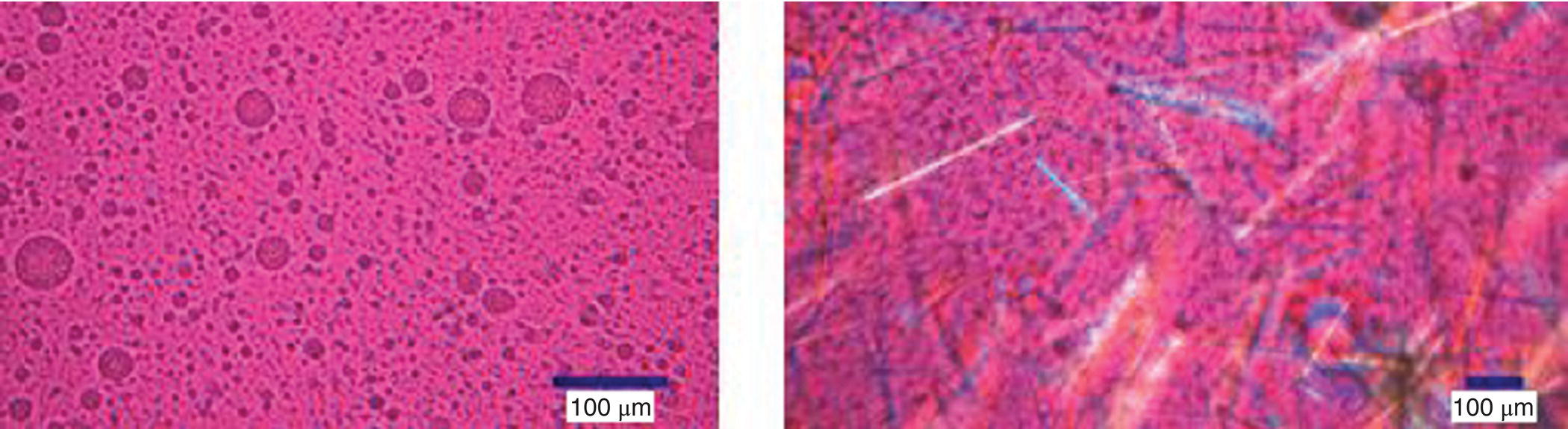
FIGURE 18.15 Illustration of data points in three‐phase triangular region.

FIGURE 18.16 Complete experimental ternary phase diagram for PDLLA/everolimus/acetone at 25 °C. ( ) points represent the boundary between two‐phase and three‐phase regions.
It is worth reiterating that the accurate determination of boundaries between 3‐ and 2‐phase regions is affected by the experimental constraints imposed by the system behavior, wherein everolimus precipitates out at lower acetone content. As a consequence, well‐spread‐out points could not be accessed to establish the vertices of the triangle, and hence, a higher level of uncertainty exists in the boundaries of the triangle.
18.5.3 Conclusions
The miscibility behavior of acetone with PDLLA and everolimus and free energy of mixing for the three components is such that a “concave‐up”‐shaped phase diagram is obtained. The diagram presents a complex phase landscape, characterized by two 1‐phase regions, three biphasic regions, and most importantly one 3‐phase region.
The manufacturing process for spraying the film onto the BVS starts with an equal weight % solution of everolimus and PDLLA in acetone, which is subsequently “dried” to remove acetone. A vertical line along the vertex of the TPD can be drawn to represent the trajectory of this film‐forming process. The trajectory suggests that between the start as a single‐phase, homogeneous solution and the end as a phase‐separated biphasic film; the system goes through at least two additional transitions. As the immiscibility curve is approached through the removal of acetone, a biphasic mixture composing of a PDLLA‐rich phase and an acetone‐rich phase is formed. Continued removal of acetone results in the formation of an additional everolimus‐rich phase as the system enters the 3‐phase triangle. Further removal of acetone results in continuous depletion of acetone‐rich phase with redistribution of its contents in the PDLLA‐ and everolimus‐rich phases. When almost all the acetone is removed, the acetone‐rich phase disappears, leaving behind a biphasic system composing of polymer‐rich and everolimus‐rich phases at the base of the phase diagram. Consistent properties of the film could be best achieved if the kinetics of the process is well controlled or the process is operated close to equilibrium during the key transitions to the biphasic film.
18.6 POLYMER–PLASTICIZER MIXING PERFORMANCE IN THE PRESENCE OF WATER
18.6.1 Introduction
The ability for polymers and additives to physically mix in many industrial applications is dictated by a combination of kinetic and thermodynamic factors. In the manufacture of ASD via HME, the API, polymer, and other excipients, for instance, need to be homogenously mixed to achieve content uniformity and complete solubility/dissolution of the API in the ASD excipient matrix. The presence of moisture can complicate the mixing performance depending on the hydrophilicity of the materials. Water may also be intentionally added as part of the process. Polymer–plasticizer mixing performance can therefore be altered by the interfacial interactions and wetting behavior between the components due to moisture. In this case study [45], a model polymer and various plasticizers were evaluated for their mixing performance in the presence of water.
18.6.2 Physical Mixing
A ternary system consisting of a polymer (copovidone, a copolymer of vinyl pyrrolidone [poly(vinyl pyrrolidone)] and vinyl acetate), a plasticizer, and water was examined for physical mixing performance. Three different liquid plasticizers (Figure 18.17) representing a range of hydrophilic–lipophilic properties characterized by their hydrophilic–lipophilic balance (HLB) and viscosities were studied (Figure 18.18). Copovidone is a hygroscopic copolymer, with a water uptake of more than 41% wt/wt at 90% RH (Figure 18.19), when measured by dynamic vapor sorption (DVS) from Surface Measurement Systems, United Kingdom. Among the plasticizers, Tween 80 (PEG‐20 sorbitan monooleate) is more hygroscopic than Span 20 (sorbitan monolaurate), and Lauroglycol FCC (propylene glycol monolaurate type I) is least hygroscopic. Span 20 is the most viscous with viscosity at 25 °C approximately 7 times higher than Tween 80. On the other hand, Lauroglycol FCC has a viscosity approximately 20 times lower than Tween 80.
FIGURE 18.17 Chemical structures of (a) Tween 80, (b) Span 20, and (c) Lauroglycol FCC.
FIGURE 18.18 HLB and viscosity values at 25 °C of the model plasticizers.

FIGURE 18.19 Water sorption isotherms for copovidone, Tween 80, Span 20, and Lauroglycol FCC at 25 °C.
Copovidone was equilibrated to different moisture contents and then physically mixed with each individual plasticizer in a ratio of 10 : 1 w/w at 25 °C to achieve a consistent mixture. The polymer–plasticizer mixing performance was directly quantified through characterization of the surface of each moisture‐equilibrated primary component (polymer and plasticizers) and polymer–plasticizer binary mixtures using inverse gas chromatography. The studies identified the following mixing behavior:
- For Lauroglycol FCC, mixing performance was independent of moisture level in copovidone.
- For Span 20, lower moisture level promoted mixing performance.
- For Tween 80, higher moisture level promoted mixing performance.
Gibbs free energy of mixing and other thermodynamic and kinetics factors were evaluated to understand these findings.
18.6.3 Gibbs Free Energy of Mixing
The thermodynamic mixing behavior of the polymer–plasticizer–water ternary system was estimated by applying the well‐known Flory–Huggins model. In the Flory–Huggins model for ternary systems, ΔGmix is made up of entropic and enthalpic terms as given by Eq. (18.4):
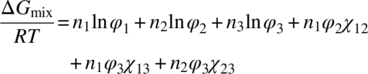
where
- n is mole fraction.
- φ is volume fraction.
- χxy is binary Flory–Huggins interaction parameter between components x and y.
- R is universal gas constant.
- T is temperature.
The subscripts 1, 2, and 3 denote water, plasticizer, and copovidone, respectively. Since Gibbs free energy of mixing, ΔGmix, is a quantitative measure of mixing tendency between components, a negative ΔGmix implies thermodynamic favorability, leading to spontaneous mixing and system stability. Some of the relevant parameters for the three components are captured in Table 18.7.
TABLE 18.7 Material Parameters for Input into the Flory–Huggins Model
| Material | Density (g/cm3) | Molecular Weight (g/mol) | Molecular Volume (cm3/mol) |
| Span 20 [46] | 1.03 | 346.5 | 5.6 × 10⁻²² |
| Tween 80 [47] | 1.08 | 1310 | 2.0 × 10⁻²¹ |
| Lauroglycol FCC [48] | 0.93 | 258.4 | 4.6 × 10⁻²² |
| Copovidone | 1.21 | 39 800 | 5.5 × 10⁻²⁰ |
| Water | 1.00 | 18.0 | 3.0 × 10⁻²³ |
Binary Flory–Huggins interaction parameters χxy between water–polymer, water–plasticizer, and polymer–plasticizer can be determined by comparing experimental and calculated water sorption isotherms of the individual components and mixtures [49, 50]. The calculated moisture sorption can be constructed using Eq. (18.5) [51, 52], with the assumption that absorption of water into the polymer or plasticizer can be treated as a dissolution process:
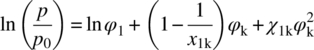
Here, subscripts 1 and k refer to water and the individual component (copovidone, Span 20, Tween 80, or Lauroglycol FCC), respectively. φk is the volume fraction of component k. The term χ1k is the binary Flory–Huggins interaction parameter dictating the strength of the interaction between water and component k. The term p/p0 is ratio of the partial vapor pressure of moisture to the saturated vapor pressure (i.e. RH%). x1k is the relative molecular volumes between water and component k.
For the “dissolution” assumption to hold, application of the above model is most appropriate at high relative humidities where the moisture is able to sufficiently plasticize the sample such that its glass transition temperature (Tg) is near or below the experimental temperature (25 °C). As a reasonable assumption, focus was therefore placed on the moisture sorption results at 80 and 90% RH to estimate the interaction parameter. Using these two data points, a value of around 0.8 was obtained for water–copovidone interaction parameter. The value, being greater than the critical value of 0.5 for polymer solutions [47], suggests that the mixing of copovidone with water is somewhat unfavorable. The unfavorability is most likely due to the hydrophobic (polyvinyl acetate) component of copovidone, because for the pure hydrophilic component (polyvinylpyrrolidone [PVP]), the interaction parameter has been reported as 0.36 [49].
The aqueous interaction parameters for the individual plasticizers were estimated as follows: the weight change due to water uptake from the moisture sorption isotherm in Figure 18.18 is first converted to water volume fraction φ1. The interaction parameter between water and component k, χ1k, is then estimated by fitting the DVS moisture sorption profile to Eq. (18.5). Results for binary interactions are tabulated in Table 18.8. With increasing hydrophobicity (in the order of Tween 80, Span 20, and Lauroglycol FCC), the interaction parameter increases due to the decreasing hygroscopicity. Additionally, positive interaction parameters for all the plasticizers indicate unfavorable mixing tendency with water.
TABLE 18.8 Flory–Huggins Interaction Parameters Determined from Moisture Sorption Isotherms
| System | Interaction Parameter (Estimated) |
| Copovidone–water | 0.8 |
| Tween 80–water | 1.0 |
| Span 20–water | 1.5 |
| Lauroglycol FCC–water | 3.6 |
For a ternary system, assuming that the water–copovidone and water–plasticizer interactions in the ternary system are the same as in the binary systems, Eq. (18.5) can be extended [49], whereby the moisture sorption profile of the plasticizer–copovidone mixture can be described by

The subscripts 1, 2, and 3 refer to water, plasticizer (Span 20, Tween 80, or Lauroglycol FCC), and copovidone, respectively, as defined above. χ23 is the binary Flory–Huggins interaction parameter dictating the strength of the interaction between the plasticizer and copovidone. If the binary interaction parameters between water and individual components are known, then the interaction parameter between the plasticizer and copovidone, χ23, can be predicted from the moisture sorption profile of the binary plasticizer–copovidone mixture using Eq. (18.6).
Experimental moisture sorption data of the copovidone–plasticizer mixtures was used to (i) confirm the presence of the copovidone–plasticizer interactions and (ii) determine if Eq. (18.6) is required to determine χ23. First, a theoretical isotherm was calculated using weighted sum of the individual components isotherm. Second, the calculated isotherm was compared against the experimental DVS moisture sorption isotherm. The presence of any copovidone–plasticizer interactions would lead to deviations between calculated and experimental profiles. However, it was found that the water uptake properties of the individual components were not altered in the physical mixtures, and therefore, no significant interaction existed between the copovidone and plasticizer (i.e. χ23 ≈ 0). In essence, the last enthalpic term of Gibbs free energy (Eq. 18.4) is reduced to zero. Furthermore the binary interaction parameters (χ12) obtained from moisture sorption isotherms (Table 18.8) are sufficient to calculate the free energy of mixing as a function of copovidone, plasticizer, and water composition using Eq. (18.4).
18.6.4 Thermodynamic and Kinetic Considerations to Mixing Behavior
The Gibbs free energy of mixing can be calculated for all copovidone, plasticizer, and water compositions at 25 °C using Eq. (18.4), from the binary interaction parameters provided in Table 18.8 and assuming no interaction between the copovidone and plasticizer (i.e. χ23 ≈ 0). The resulting Gibbs free energy of mixing is shown as ternary diagrams in Figure 18.20. The lowest free energies are achieved at low water content, indicating that mixing between copovidone and plasticizer is more favorable when moisture is minimized. Free energy contour lines in the system involving Tween 80 are less dependent on the copovidone and plasticizer compositions than in the systems involving Span 20 and, especially, Lauroglycol FCC. This is due to relatively similar interaction parameters between water–copovidone (χ13 = 0.8) and water–Tween 80 (χ12 = 1.0). In other words, physical mixing is most sensitive to copovidone and plasticizer compositions for Lauroglycol FCC and least sensitive for Tween 80. These results also show that for a more hydrophobic plasticizer (with lower HLB value), increasing water results in decreased mixing favorability.
FIGURE 18.20 Contour lines of the Gibbs free energy of mixing for the ternary systems of copovidone, plasticizer, and water. Plasticizers are (a) Tween 80, (b) Span 20, and (c) Lauroglycol FCC.
Comparison of this predicted mixing performance to the experimental results, however, shows that physical mixing behavior was not solely influenced by thermodynamic factors, since Lauroglycol FFC displayed the best mixing performance regardless of water content. Kinetic barrier could also be very important. Lauroglycol FCC has low kinetic barrier because its viscosity is one and two orders of magnitude lower than Tween 80 and Span 20, respectively. The relatively low viscosity of this plasticizer would allow it to be easily incorporated into the copovidone regardless of the moisture content. It is also interesting to note that when kinetic barriers are high due to high viscosity such as for Tween 80, mixing performance is dictated by more favorable interactions with water. For viscous polymers, the study therefore shows that underlying thermodynamic characteristics become more dominant for mixing favorability.
18.6.5 Conclusions
The mixing of polymers and additives in the presence of water is dictated by a combination of kinetic and thermodynamic factors; this arises from material physical properties, such as viscosity, hydrophobicity (surface properties), and moisture uptake behavior. As the viscosity of the components decreased in the system, the influence of the thermodynamic characteristics became less important. In summary, the Flory–Huggins model and ΔGmix calculations provide a quick and quantitative estimation of performance for industrial mixing applications between polymer and surfactant at different water contents.
REFERENCES
- 1. Haleblian, J. and McCrone, W. (1969). Pharmaceutical applications of polymorphism. J. Pharm. Sci. 58: 911–929.
- 2. Rodriguez‐Spong, B., Price, C.P., Jayasankar, A. et al. (2004). General principles of pharmaceutical polymorphism: a supramolecular perspective. Adv. Drug Deliv. Rev. 56: 241–274.
- 3. Cruz‐Cabeza, A., Reutzel‐Edens, S.M., and Bernstein, J. (2015). Facts and fictions about polymorphism. Chem. Soc. Rev. 44: 8619–8635.
- 4. Almarsson, Ö. and Zaworotko, M.J. (2004). Crystal engineering of the composition of pharmaceutical phases. Do pharmaceutical co‐crystals represent a new path to improved medicines? Chem. Commun. 1889–1896.
- 5. Vishweshwar, P., McMahon, J.A., Bis, J.A., and Zaworotko, M.J. (2006). Pharmaceutical cocrystals. J. Pharm. Sci. 95: 499–516.
- 6. Friscic, T. and Jones, W. (2010). Benefits of co‐crystallization in pharmaceutical material science – an update. J. Pharm. Pharmacol. 62: 1547–1559.
- 7. Thakuria, R., Delori, A., Jones, W. et al. (2013). Pharmaceutical co‐crystals and poorly soluble drugs. Int. J. Pharm. 453: 101–125.
- 8. Crane, I.M., Mulhern, M.G., and Nema, S. (2003). Stability of reconstituted parecoxib for injection with commonly used diluents. J. Clin. Pharm. Therap. 28: 363–369.
- 9. Sheikh, A.Y., Borchardt, T.B., Ferro, L.J., and Danzer, G.D. (2003). Crystalline parecoxib sodium. US Patent US20030232871.
- 10. Morris, K.R., Griesser, U.J., Eckhardt, C.J., and Stowell, J.G. (2001). Theoretical approaches to physical transformations of active pharmaceutical ingredients during manufacturing processes. Adv. Drug Deliv. Rev. 48: 91–114.
- 11. Oliveira, M.A., Peterson, M.L., and Davey, R.J. (2011). Relative enthalpy of formation for co‐crystals of small organic molecules. Cryst. Growth Des. 11: 449–457.
- 12. Grant, D.J.W. and Higuchi, T. (eds.) (1990). Dissolution rates of solids. In: Solubility Behavior of Organic Compounds, Techniques of Chemistry, vol. 21, 474–551. New York: Wiley.
- 13. Bernstein, J., Davey, R.J., and Henck, J. (1999). Concomitant polymorphs. Angew. Chem. Int. Ed. 38: 3440–3461.
- 14. Yu, L. (1995). Inferring thermodynamic stability relationship of polymorphs from melting data. J. Pharm. Sci. 84: 966–974.
- 15. Yu, L., Huang, J., and Jones, K.J. (2005). Measuring free‐energy differences between crystal polymorphs through eutectic melting. J. Phys. Chem. B 109: 19915–19922.
- 16. McCrone, W. (1957). Fusion Methods in Chemical Microscopy: A Textbook and Laboratory Manual. New York: Interscience Publishers.
- 17. Ku, Y., McDaniel, K.F., Chen, H.‐J. et al. (2010). Preparation of heterocyclic macrocyclic peptides as hepatitis C serine protease inhibitors. International Patent WO 2010/030359 A2.
- 18. Liepold, B., Moosmann, A., Pauli, M. et al. (2015). Solid pharmaceutical compositions useful in HCV treatment. International Patent WO 2015/071488 A1.
- 19. Sun, Y., Tao, Z., Zhang, G.Z.Z., and Yu, L. (2010). Solubilities of crystalline drugs in polymers: an improved analytical method and comparison of solubilities of indomethacin and nifedipine in PVP, PVP/VA and PVAc. J. Pharm. Sci. 99: 4023–4031.
- 20. Sheikh, A.Y., Diwan, M., Pal, A.E. et al. (2014). Crystalline forms of an HCV protease inhibitor. International Patent WO 2014/011840 A1.
- 21. Brackemeyer, P.J., Diwan, M., Gong, Y. et al. (2015). Crystal form of ABT 450. International Patent WO 2015/084953 A1.
- 22. Hong, G.‐B., Lee, M., and Lin, H. (2002). Liquid‐liquid equilibrium of ternary mixtures of water‐2‐propanol with ethyl acetate and isopropyl acetate or ethyl caproate. Fluid Phase Equilib. 202: 239–252.
- 23. Walsh, R., Bradner, M.W., Fleischman, S.G. et al. (2003). Crystal engineering of the composition of pharmaceutical phases. Chem. Commun. 186–187.
- 24. Nehm, S.J., Rodriguez‐Spong, B., and Rodriguez‐Hornedo, N. (2006). Phase solubility diagrams of cocrystals are explained by solubility product and solution complexation. Cryst. Growth Des. 6: 592–600.
- 25. Trask, A.V., Streek, J.V.D., Motherwell, W.D.S., and Jones, W. (2005). Achieving polymorphic and stoichiometric diversity in cocrystal formation: importance of solid‐state grinding, powder X‐ray structure determination, and seeding. Cryst. Growth Des. 5: 2233–2241.
- 26. Etter, M.C. and Reutzel, S.M. (1991). Hydrogen bond directed cocrystallization and molecular recognition properties of acyclic imides. J. Am. Chem. Soc. 113: 2586–2598.
- 27. Chadwick, K., Davey, R.J., and Cross, W. (2007). How does grinding produce co‐crystals? Insights from the case of benzophenone and diphenylamine. CrystEngComm 9: 732–734.
- 28. Seefeldt, K., Miller, J., Alvarez‐Nunez, F., and Rodriguez‐Hornedo, N. (2007). Crystallization pathways and kinetics of carbamazepine–nicotinamide cocrystals from the amorphous state by in situ thermomicroscopy, spectroscopy, and calorimetry studies. J. Pharm. Sci. 96: 1147–1158.
- 29. Zhang, G.G.Z., Henry, R., Borchardt, T.B., and Lou, X.C. (2007). Efficient co‐crystal screening using solution‐mediated phase transformation. J. Pharm. Sci. 96: 990–995.
- 30. Mullin, J.W. (ed.) (2001). Crystallizer design and operation. In: Crystallization, 4e, 315–402. Oxford: Butterworth‐Heinemann.
- 31. Sheikh, A.Y., Abd, R.S., Hammond, R.B., and Roberts, K.J. (2009). Scalable solution cocrystallization: case of carbamazepine‐nicotinamide I. CrystEngComm 11: 501–509.
- 32. Chiarella, R.A., Davey, R.J., and Peterson, M.L. (2005). Making co‐crystals – the utility of ternary phase diagrams. Cryst. Growth Des. 5: 2233–2241.
- 33. Lange, L. and Sadowski, G. (2015). Thermodynamic modeling of efficient co‐crystal formation. Cryst. Growth Des. 15: 4406–4416.
- 34. Rapoza, R., Veldhof, S., Oberhauser, J., and Hossainy, S.F.A. (2015). Assessment of a drug eluting bioresorbable vascular scaffold. US Patent 2015/0073536 A1.
- 35. Tarantini, G., Masiero, G., Granada, J.F., and Rapoza, R.J. (2016). The BVS concept, from the chemical structure to vascular biology; the bases for a change in interventional cardiology. Minerva Cardioangiol. 64: 419–441.
- 36. Kossuth, M.B., Perkins, L.E.L., and Rapoza, R.J. (2016). Design principles of bioresorbable polymeric scaffolds. Interv. Cardiol. Clin. 5: 349–355.
- 37. Rapoza, R., Ding, N., Wang, Y. et al. (2014). Bioresorbable implants for transmyocardial revascularization. US Patent 2014/0336747 A1, 13 November 2014.
- 38. Chen, Y., Van Sciver, J., Hossainy, S.F.A., and Pacetti, S.D. (2010). Drying bioresorbable coating over stents. US Patent 20100323093 A1.
- 39. Wu, M., Kleiner, L., Tang, F.W. et al. (2010). Surface characterization of poly(lactic acid)/everolimus and poly(ethylene vinyl alcohol)/everolimus stents. Drug Deliv. 17: 376–384.
- 40. Hossainy, S.F.A. (2015). Phase separated block co‐polymer coatings for implantable medical devices. US Patent US 2015/9028859 B2, 12 May 2015.
- 41. Fox, T.G. and Flory, P.J. (1950). Second‐order transition temperatures and related properties of polystyrene. J. Appl. Phys. 21: 581–591.
- 42. Shefter, E. and Higuchi, T. (1963). Dissolution behavior of crystalline solvated and non‐solvated forms of some pharmaceuticals. J. Pharm. Sci. 52: 781–791.
- 43. Nakafuku, C. and Takeshia, S. (2004). Glass transition temperature and mechanical properties of PLLA and PDLLA‐PGA co‐polymer blends. J. App. Polym. Sci. 93: 2164–2173.
- 44. Duffy, J.D., Stidham, H.D., Hsu, S.L. et al. (2002). Effect of polyester structure on the interaction parameters and morphology development of ternary blends: model for high performance adhesives and coatings. J. Mater. Sci. 37: 4801–4809.
- 45. Ho, R., Sun, Y., and Chen, B. (2015). Impact of moisture and plasticizer properties on polymer–plasticizer physical mixing performance. J. Appl. Polym. Sci. 132: 41679–41688.
- 46. Gangolli, S. (1999). The Dictionary of Substances and Their Effects: Volume 6 O‐S, 2e. Cambridge, UK: Royal Society of Chemistry.
- 47. Ravve, A. (2012). Principles of Polymer Chemistry, 3e. New York: Springer.
- 48. Gattefosse (2010). Technical data sheet: lauroglycol FCC, Specification number 3219/5.
- 49. Rumondor, A.C.F. (2010). Analysis of the moisture sorption behavior of amorphous drug–polymer blends. J. Appl. Polym. Sci. 117: 1055–1063.
- 50. Crowley, K.J. and Zografi, G. (2002). Water vapor absorption into amorphous hydrophobic drug/poly(vinylpyrrolidone) dispersions. J. Pharm. Sci. 91: 2150–2165.
- 51. Flory, P.J. (1942). Thermodynamics of high polymer solutions. J. Chem. Phys. 10: 51–61.
- 52. Hancock, B. and Zografi, G. (1993). The use of solution theories for predicting water vapor absorption by amorphous pharmaceutical solids: a test of the Flory‐Huggins and Vrentas models. Pharm. Res. 10: 1262–1267.