
26
MEASUREMENT OF SOLUBILITY AND ESTIMATION OF CRYSTAL NUCLEATION AND GROWTH KINETICS
Nandkishor K. Nere, Manish S. Kelkar, Ann M. Czyzewski, Kushal Sinha, and Evelina B. Kim
Process Research and Development, AbbVie Inc., North Chicago, IL, USA
26.1 INTRODUCTION
The performance of a crystallization process in terms of the resulting particle size distribution and impurity rejection is largely dictated by the relative rates of crystal nucleation and growth. Hence, characterization of nucleation and growth kinetics is of paramount importance to enable the efficient development of robust crystallization processes. The fundamental basis on which to understand any crystallization process is solubility; this chapter begins with a discussion of solubility measurement methodologies, best practices, and relevant examples. We then delve into a discussion of different approaches to interrogating nucleation and growth kinetics, including both experimental and computational methodologies. Lastly, relevant case studies are presented to exemplify how a fundamental understanding of nucleation and growth kinetics can be used in the development of an appropriate crystallization process and control strategy.
26.2 SOLUBILITY
The term solubility is defined as “analytical composition of a mixture or solution, which is saturated with one of the components of the mixture or solution, expressed in terms of the proportion of the designated component in the designated mixture or solution” [1]. While the “mixture” or “solution” could be composed of any physical state, this discussion is focused on systems in which a crystalline solid (solute) is dissolved in a liquid (solvent), as those pertain to industrial crystallizations of drug substances (DSs) and/or their chemical intermediates.
When a solid is contacted with a liquid, a dynamic process is initiated wherein molecules from the solid phase dissolve into the liquid phase and dissolved molecules re‐adsorb onto the solid surface. Initially, the rate of solute molecules going into the liquid phase is higher than that of solute molecules adsorbing back on the solid surface, resulting in increased concentration of solute in the solution. Eventually, a dynamic equilibrium is reached, where the rates of dissolution and adsorption are equal, and the solute concentration reaches a steady state. This concentration is defined as the solubility of the solute in a given solvent. For any solute A, this equilibrium can be depicted as
where
- A(S) is solute in solid phase.
- A(L) is solute in liquid phase.
- μ(A, S) is the chemical potential of A in solid phase S.
- μ(A, L) is the chemical potential of A in liquid phase L.
This solid–liquid equilibrium can be mathematically represented by the van’t Hoff equation as

where
- ∆Hm is the molar enthalpy of melting.
- R is the universal gas constant.
- Tm is the absolute melting temperature of the solute.
- T is the absolute temperature of the solution.
- x is the mole fraction of the solute.
- γ is the activity coefficient.
As solubility is significantly influenced by properties of both the solvent and solute, characterization of the solid phase is very important for accurate definition and measurement of solubility.
Discussed in this section are several of the more prevalent methods used to measure solubility as the first step toward the goal of developing commercializable crystallization processes for pharmaceutical compounds. Measurements near the critical region, under high pressures, or advanced methods used in bioavailability/pharmacokinetic studies and during drug discovery phase are not discussed here.
26.2.1 Shaker‐Flask Method
Typically, measurement of solubility involves some variation of the shaker‐flask method and includes the following steps:
- Solid–liquid contact and attainment of equilibrium.
- Sampling or separation of solid and liquid phases.
- Measurement of solute concentration in liquid phase.
- Confirmation of crystal form of the solid phase.
Some considerations for obtaining accurate solubility measurements in the context of the shaker‐flask procedure are outlined in the following subsections.
26.2.1.1 Material Properties
26.2.1.1.1 Purity
The presence of very small amounts of impurities in a solubility study can significantly affect the measured solubility. Impurities can not only change the activity coefficient in Eq. (26.3), thus altering the solubility of solute significantly, but in some cases, they can also alter the thermodynamic stability of the solute solid form. Impurities can also impact nucleation and growth kinetics, which can in turn affect the solubility measurement.
To ensure the most accurate and representative solubility measurements are obtained, it is important to avoid contamination with extraneous impurities and ensure the system is stable such that degradants do not form over time. It is equally important to interrogate the impact of process‐related impurities on the measured solubility when relevant to the system being evaluated.
26.2.1.1.2 Effect of Solute Content and Particle Size
The amount of solute present in a solubility experiment should be sufficient to ensure it will not completely dissolve over the time course of the study and have enough solids to evaluate crystal form while not using an excessive amount, making it hard to mix. In certain situations, such as in the case of indomethacin [2], the amount of suspended solid could affect the measured solubility due to an imbalance between solute crystallization and dissolution rates. It is recommended that the amount of solute present in the experiment be reported and, if necessary, the impact of solute amount on measured solubility be explored.
Studies have also shown the effect of particle size on the measured solubility through Gibbs–Thomson type of equation [3]:

where
- c(r) is solubility of solid with particle radius of r.
- c* is the equilibrium solubility of the solid substance.
- M is the molar mass of solid in solution.
- γ is the interfacial tension of solid and liquid.
- ρ is the density of the solid.
- ϑ is the number of moles of ions generated from 1 mol of solute.
For nonionic substance, ϑ = 1. Ratios [c(r)/c*] of as high as approximately 13 have been observed in the literature for some inorganic compounds [3].
26.2.1.2 Experimental Setup and Design
Important considerations for appropriate equipment setup and design include material compatibility, agitation design, and approach and attainment of equilibrium.
26.2.1.2.1 Material Compatibility
The compatibility of the system (solute and solvent) with the container and sampling device needs to be considered. In general, glass vials/reactors are used on account of their reasonable chemical inertness. Vials should be tightly sealed to avoid evaporation of solvent (especially when dealing with solvent mixtures) and exposure to air/oxygen/moisture. If the study materials are photosensitive, exposure to light should be reduced by using dark/amber‐colored vials or by keeping the vials in dark container.
26.2.1.2.2 Agitation
Agitation promotes intimate contact between solid and liquid phases, which is required to facilitate proper wetting of the solids and equilibration of the two‐phase system. Several types of equipment (rocking table, vortex mixer, mechanical arm, etc.) can be used to keep the solubility vial in motion, thus providing mixing. Typically, this type of mixing is expected to be gentler on the crystals and is employed when solubility screening is coupled with crystal morphology screening. Alternatively, an overhead stirrer or magnetic stirrer can be used to internally agitate the solubility mixture rather than relying on the motion of the container to contact the phases. This type of mixing is usually more vigorous and can accelerate attainment of equilibrium, which is especially useful in the systems with slow dissolution/de‐supersaturation kinetics. However, it should be noted that magnetic stirrers can grind the solids, thus impacting the resultant crystal morphology, particle size, and crystallinity to some extent.
26.2.1.2.3 Approach and Attainment of Equilibrium
During the equilibration period, the solubility can be approached by either (i) dissolving more solute in an undersaturated solution (saturation experiment) or (ii) removing solute from a supersaturated solution (de‐supersaturation experiment). Schematically, these approaches to equilibrium solubility are represented in Figure 26.1. Since theoretically both approaches should result in the same value, it is recommended that solubility measurements be made both ways as a means of verification. A difference in measured values from these two approaches may indicate that impurities are impacting solubility or de‐supersaturation kinetics. This impact can be further discerned by repeating the approach from undersaturation experiments in the presence of spiked impurities (one at a time) and measuring solubility. A difference in the measured solubility may confirm the impurity’s impact on solubility, while a similar value may indicate an effect of an impurity on crystallization kinetics of the solute.

FIGURE 26.1 Schematic demonstrating an approach to equilibrium solubility from (a) undersaturation and (b) supersaturation.
The attainment of equilibrium in a two‐phase system takes time, typically on the order of hours to days of sustained intimate contact. The time needed to reach equilibrium can vary based on liquid and solid physical properties as well as experimental conditions; however, equilibrating mixtures for 24 hours before sampling for solubility measurements is recommended. Best practice is to take at least two consecutive measurements, which should measure within experimental error, to confirm equilibrium has been reached. Moreover, care must be taken to ensure equilibrium is not disturbed during the hold period by, for example, adding new solvent to the mixture or exposing the system to variable temperatures. Lastly, it is very important that the solute is chemically stable throughout the duration of the hold period so as to avoid impact of the degradants on the solubility measurements (see Section 26.2.1.1).
26.2.1.3 Equilibration Parameters
Two of the most notable parameters that can significantly impact solubility measurements in a given solvent system are temperature and pH. The impact of temperature on solubility in different systems can vary significantly; however, it has been reported that, for example, controlling temperature to within ±1 °C for an organic compound with a heat of solution of approximately 10 kcal/mol leads to variability in measured solubility of about ±10% [4]. Best practice, therefore, is to accurately control temperature to the extent possible both during the equilibration and during the sampling for solubility measurements.
The pH of a mixture can impact solubility (particularly salts) as well as the distribution of ionic species and hence the crystal form of the solid. It is notable that solubility of a salt can also be affected by the choice of acid/base through the common ion effect, particularly at extremes of the pH scale. Artificially low solubility may be observed due to salting out of the desired compound due to the presence of common ions introduced through acids or bases.
26.2.1.4 Sampling
The conventional sampling method involves removing a sample for solubility measurement. After allowing the solids to settle as much as possible, a sample of the liquid phase is removed and filtered through an appropriate microporous disposable syringe filter (0.2 or 0.45 μm). It is important to ensure that the selected filters do not adsorb the solute and are used correctly in order to not adversely impact the solubility measurement. Using this sampling method, it can be difficult to maintain equilibrium conditions throughout isolation of the sample, particularly at high and low temperatures. Typically, syringes/probes used to sample slurries/liquids are preheated/precooled to appropriate temperature to avoid disturbing the equilibrium while sampling. On the other hand, this challenge can also be overcome using automated sampling techniques discussed below.
Sampling robots or auto‐sampling assemblies, such as Global FIA® FloPro® and Komplx® KS‐1, can be used efficiently to sample systems with minimal disturbance to equilibration. These sampling systems can automatically filter a slurry and sample only the mother liquor, making them useful for tracking de‐supersaturation. Most sampling systems can also automatically quench or dilute the samples to ensure the composition does not change over time. The Komplx® KS‐1 system has the ability to dilute the sample at the probe, and FloPro® has introduced heated probes, both enhancements that can further minimize temperature effects during sampling.
In isosystic systems, where analysis is performed with in situ probes/process analytical tools (PAT), external sampling of slurry or mother liquor is not necessary. In such cases, disturbance of the system equilibrium is minimized. These systems are particularly useful in data intensive studies, wherein sample preparation and analysis can become burdensome.
26.2.1.5 Measurement of Solute Concentration in Liquid Phase
Many different destructive and nondestructive methods can be used to analyze solute concentration in the liquid phase. Some of the most commonly used techniques used for solubility measurements are described in the subsections below. The simplest method to analyze the liquid‐phase concentration is to evaporate a known quantity of well‐characterized solvent and quantitate the resultant solid residue. Alternatively, solute can be added incrementally to a solution to approximate the solubility limit. These methods are inexpensive and do not need elaborate method development; however, they are only useful for approximate quantitation.
26.2.1.5.1 Chromatographic Methods
Chromatography (HPLC/UPLC or GC) is one of the most common methods used to measure solute concentration. The mother liquor sample is diluted in prescribed diluent and is then analyzed using a predefined method that can separate the substrate of interest from impurities. While these methods are quantitatively very accurate, these methods require appropriate chromatographic method development and sample preparation, which could be labor intensive. These methods may not be ideal for high‐throughput solubility measurements; however, autosampling robots and online HPLC systems can help circumvent some of these challenges.
26.2.1.5.2 In Situ Methods
Various in situ measurement methods such as electrical methods (conductometry, electromotive force, polarography, pH), optical methods (colorimetry, refractometry, polarimetry), spectrophotometric methods (UV/Vis, infrared [IR], near IR [NIR], Raman), and densitometry can be employed to determine the concentration of the solute in solution. The selectivity and sensitivity of these nondestructive methods (including impact of impurities) need to be evaluated for each of the solubility measurement systems. Quantitative solubility determination requires development of a calibration curve. When applicable, these high‐throughput methods are ideal for solubility screening as they are able to generate large amounts of data that can inform solubility behavior.
26.2.1.6 Confirmation of the Crystal Form of the Solid Phase
As solubility is defined with respect to a specific solid crystal form, the solid form of the equilibrated solids is typically analyzed using a powder X‐ray diffractometer (XRD) and compared to reference patterns. Solids can be isolated using disposable or fritted centrifuge tubes, and the wet cake prepared for X‐ray powder diffraction (XRPD) analysis. Due to the potential for solid form to change during isolation and drying, it is best to analyze a wet cake rather than fully dried solids. High‐throughput XRD machines are available to efficiently screen a large number of samples (e.g. Bruker’s D8 Discover HTS2 system). Other off‐line techniques such as differential scanning calorimetry (DSC) or thermogravimetric analysis DSC (TGA‐DSC) can also be used to verify solid forms based on known melting point, melting point shift, and/or mass loss (for solvates/hydrates).
In situ methods such as spectroscopic techniques including IR, NIR, or Raman can also be used to distinguish between solid forms. The applicability of such techniques for each system needs to be evaluated before the use, as interference from solvents in the region of interest may render these methods inappropriate.
26.2.2 Other Methods: Clear Point or Cloud Point Method
Methods based on cloud point or clear point determination can be an attractive alternative to the shaker‐flask method for rapid estimation of solubility. Tedious sampling and analytical method development can be avoided using these techniques because the composition of the solution is determined mathematically based on the known charge amounts of solid and liquid phases. Polythermal (plethostatic) methods entail exposing a solid/liquid mixture of known composition in a sealed vial to a temperature ramp while monitoring the turbidity of the mixture. The clear point is the temperature at which solids dissolve. While the clear point temperature is fundamentally different than the solubility temperature, it approaches the solubility temperature when the heating rate is slow relative to the kinetics of dissolution and hence can be used to estimate solubility.
Once a clear/homogeneous solution is obtained, the solution can then be cooled until it becomes cloudy, which marks the cloud point temperature. In conjunction with the clear point temperature, the cloud point temperature measurement can generate information about the metastable zone width (MSZW). As the cooling rate is decreased, the cloud point temperature approaches the clear point temperature. These temperature variation methods are reversible such that the same sample can typically be heated and cooled multiple times to get precision on the measurement provided the crystal form of the solids does not change. These methods can also be used to learn about liquid–liquid‐phase separation (LLPS) during crystallization.
Isothermal methods, on the other hand, alter the composition of the vial while holding at constant temperature until a clear solution is obtained. The composition at which the solids completely dissolve is called the clear point composition. When the solvent is added slowly enough, the clear point composition, and hence the solubility at the given temperature, can be estimated with reasonable accuracy. Unlike the temperature variation method, the solvent addition method is not reversible; fresh solvent/solute mixtures must be prepared and tested to evaluate reproducibility of the measurement.
Because these methods require less manual intervention and are amenable to automation, multi‐reactor setups such as Crystal16® and Crystalline® are well suited for these measurements. While Crystalline® can execute both temperature variation and solvent addition methods, Crystal16® is not currently designed to execute solvent addition experiments readily.
There are several considerations that can factor into the applicability of clear and cloud point measurements to a particular study. One consideration is that these methods require a priori knowledge of the approximate solubility and polymorph landscape. The experimental conditions must be selected to ensure the clear/cloud points will be traversed over the range of interest. Moreover, because solids dissolve and are not available for crystal form testing, the crystal form landscape must be understood to confirm that (i) the desired form is stable over the experimental range of the studies and (ii) no metastable forms exist. Additionally, if the dissolution kinetics are unusually slow, errors in solubility measurement can be incurred. Measurements at different temperature ramps and solvent addition rates are hence recommended to avoid erroneous conclusions. Lastly, the clear point temperature can be underestimated if the system under study is prone to “crowning,” i.e. creeping/crystallization of solid phase on the walls of the vial above the liquid level. The erroneous conclusion could also be reached if the solids tend to cream or settle readily, and the optical sensor may not detect the solids present in the experiment. This issue can be somewhat mitigated by using alkaline earth metal stir bars; however, it is a good practice to observe the vials periodically to confirm if such problems exist and rectify those in timely manner.
26.2.3 Regression of Solubility Data
Mathematical treatment of solubility data can oftentimes be insightful to garner more information from the discrete and limited measurements. During early process development, solubility data from the solvent screening can be appropriately modeled to render solubility prediction in a variety of solvents, which can significantly reduce the number of experiments. For the later stages of process development when the solvent system is already established, solubility experiments are designed to collect detailed solubility data at various process‐relevant conditions. These data are typically regressed to get a mathematical representation of solubility as a continuous function of a relevant process parameter (solvent composition, temperature, pH, etc.). The resulting solubility equation is customarily the backbone upon which the crystallization process parameters are built.
Various mathematical models have been used in the literature to fit solubility data [3]; some of the more commonly used model equations are summarized below in Table 26.1.
TABLE 26.1 Solubility Regression Models Describing Equilibrium Solubility (c*) for One‐solvent and Two‐solvent Systems
| One‐Solvent Systems | Two‐Solvent Systems | ||
| lnc* = A + BT + CT2 | (26.5) | (26.8) | |
| (26.6) | (26.9) | ||
| (26.7) | (26.10) | ||
T is the absolute temperature.
x1 is the anti‐solvent weight fraction.
A, B, C, and D are the constants/fit parameters.
For the limiting case of one solvent (x1 → 0), the model equations (26.8)–(26.10) for two‐solvent systems equations convert to a form similar to Eq. (26.6). Models represented by Eqs. (26.8)–(26.10) are also included in the Crystallization Toolbox utility from DynoChem®. This software utility can fit the measured solubility data and choose the best fit equation for further crystallization process modeling and design.
Other models, e.g. nonrandom two‐liquid segment activity coefficient (NRTL‐SAC) and UNIQUAC functional group activity coefficients (UNIFAQ), are also frequently used to model and fit the solubility data. They are included in some of the commercially available software such as Aspen Properties®.
The solubility of a salt as a function of pH is typically modeled using Henderson–Hasselbalch equation. For a monoacidic salt at a pH > pKa, this equation can be written as Eq. (26.11). Caution must be used in extrapolating this model beyond the measured pH window to account for the stability of crystal form:
Other approach‐based theories of solid–liquid equilibria also exist for the prediction of solubilities of crystalline solids in liquids and are not discussed here.
26.2.4 Recommended Protocol for Solubility Measurement
A recommended protocol for measuring solubility is summarized below. Care must be taken to use consistent units (mg/ml solution, mg/g solution, mg/g solvent, wt %) while measuring, reporting, and using the solubility data. A significant error can be introduced through the density of solution (ml vs. g) or basis of measurement (solvent vs. solution):
- Plan experiments to approach solid–liquid equilibrium from both saturation and de‐supersaturation.
- Mix the desired solid form with solvents/solutions with magnetic stir bar.
- Equilibrate at desired pH and/or temperature for approximately 24 hours if the chemical stability is not of concern and kinetics of solubilization are not known a priori.
- Confirm the presence of solids and ensure that desired temperature and/or pH along with the total mass is maintained. If not, set the system to desired state point and equilibrate for another 24 hours.
- If desired state point is maintained, sample liquid phase without disturbing the equilibrium.
- Analyze the liquid phase for concentration of the compound of interest using appropriate technique (i.e. HPLC, IR, etc.).
- Stir for another approximately 24 hours.
- Confirm that the desired state point is maintained and sample the liquid phase again.
- Analyze the liquid phase again for concentration of the compound of interest.
- If the two measured concentrations are within acceptable tolerance, sample the solid phase to confirm crystal form.
- If mixture of solvents is used, sample liquid phase (using GC, KF, etc.) for solvent composition.
- If crystal form is consistent and solvent composition is maintained, the measured concentration is the solubility at the given state point (crystal form, temperature, solvent composition, impurity profile, pH).
- Evaluate the effect of process‐relevant impurities by comparing saturation and de‐supersaturation experiments and spiking specific impurities during the solubility measurement experiments.
- Regress the data using an appropriate mathematical model to enable solubility predictions over the desired state space.
26.2.5 Example Applications of Solubility Measurement
In this section, practical examples of how the solubility measurement recommendations and best practices have been applied to crystallization process design and development are presented. The first example describes the use of a NRTL‐SAC model to develop the process. The second case illustrates the regression of solubility data using the DynoChem® Crystallization Utility. The third example showcases the use of automated lab reactors and PAT to aid in solubility measurements. The final example combines various aspects of solvent screening/detailed study, use of NRTL‐SAC, regression, and influence of the solubility on the crystallization process development.
26.2.5.1 Solubility Measurements as a Function of Temperature and Antisolvent Amount with Data Fitting Using NRTL‐SAC Model
This example summarizes the measurement of solubility data for pharmaceutical compound A, the desired form of which is a solvate hydrate. The solubility of compound A was measured in methanol as a function of water (antisolvent) content and temperature. The data were then fitted to the NRTL‐SAC model using Aspen Properties® V8.6. Figure 26.2 shows measured solubility data, and the resulting model fits for the desired crystal form (confirmed by XRPD).
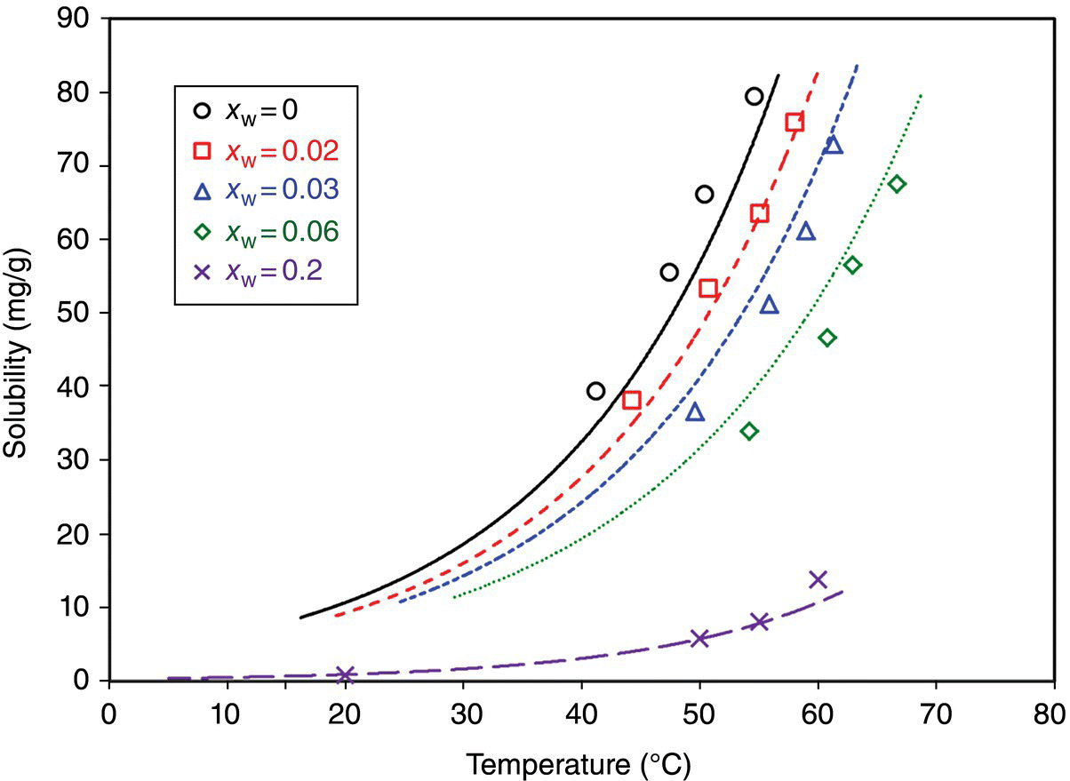
FIGURE 26.2 Raw solubility data of compound A in methanol as a function of water content (antisolvent) and temperature. xW is the weight fraction of water in the solution.
These data were the basis for designing a methanol–water antisolvent crystallization that is capable of delivering the desired yield. Furthermore, this understanding of solubility variation over the solvent composition and temperature range informed the optimal seeding conditions and helped to design the procedure used to reduce fines through Ostwald ripening.
26.2.5.2 Solvent Screening and Solubility Measurements at Different Temperatures and Regression with DynoChem®
In this example, solubility of pharmaceutical compound B was screened in different solvents and/or solvent combinations to measure how much solute could be dissolved at the given process conditions. Based on the solvent screening experiments and the choice of upstream reaction solvents, 2‐MeTHF–water–heptane system was selected. Water was a good solvent, 2‐MeTHF was a moderate solvent, and heptane was used as an antisolvent. Detailed solubility measurements were carried out for compound B in the miscibility region of 2‐MeTHF–water system with the recommended protocol (Section 26.2.4). HPLC was used to analytically measure the concentration in the solvent system. The data were then regressed using five different equations in DynoChem®, and Eq. (26.9) that yielded the best fit was selected. Figure 26.3 shows the fitted solubility as a function of water/2‐MeTHF composition and temperature.

FIGURE 26.3 Estimated solubility of compound B using best‐fit equation (Eq. (26.9) from Table 26.1) in DynoChem® as a function of water composition in a designated temperature range. (a) Parity plot for comparison between measured and predicted solubilities. (b) Estimated solubility as a function of water content (wt %) and temperature.
As can be noticed from Figure 26.3b, as water content decreases, the temperature dependence of solubility also diminishes. Similar data were also collected for 2‐MeTHF–water–heptane system (not shown here). The data helped design the amount of water that needs to be removed and amount of heptane that needs to be added for improving the yield and performance of the crystallization. The estimated data also suggest that at lower water content, the temperature dependence of solubility is nonexistent. Hence, if temperature cycling is required for reduction of fines, it would be better to carry out the temperature cycling at higher water content to take advantage of the solubility.
26.2.5.3 Solubility Measurement with EasyMax® and Online HPLC
Solubility of compound C was measured in ethyl acetate as a function of temperature. The data were collected from the experiments conducted in a 100 ml automated reactor using an online HPLC system.
The solubility of compound C was screened in different solvents, and ethyl acetate was picked as the solvent of choice. More elaborate solubility measurements were then carried out to further understand the crystallization process and impact on the impurity rejection. Crude C was suspended in ethyl acetate such that representative impurities would be present in the system. 100 ml Mettler Toledo® EasyMax® reactor was used with overhead stirring to simulate representative process conditions. The automated reactor was fitted with an online HPLC probe (KS‐1 from Komplx®). The probe is designed to sample the mother liquor (ML) of the slurry by filtering it through a Teflon filter and diluting it immediately with the prescribed diluent and then running it automatically on the HPLC.
The system was programmed to equilibrate at different temperatures from 0 °C up to 75 °C. The system was equilibrated for 4 hours at each temperature, and sampling was carried out every 30 min. Compound C was studied a priori to ensure the stability of the desired crystal form under explored temperature range in ethyl acetate. The system was also cooled back down to 0 °C while equilibrating at the same temperatures as used during ramp up. The data are summarized in Figure 26.4. As can be seen from the data, four hours was enough to reach equilibration for this system during heating. It can also be seen that during cooldown, as temperature decreased, the time required to reach equilibrium increased.
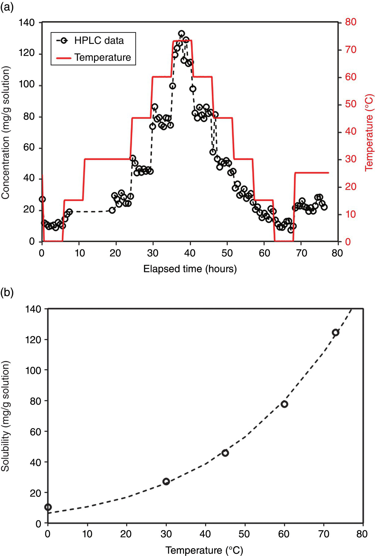
FIGURE 26.4 (a) Raw data of solubility and temperature collected in an automated reactor using online HPLC. (b) Summarized solubility data with an exponential model fit for the solubility.
Measured solubility data were useful to understand the impact of temperature and ethyl acetate charge on the yield of the process. As crude solids for compound C were used with representative impurities, online HPLC could be used to determine the purge of impurities in the ML at various temperatures. The data were also used to understand the rate of de‐supersaturation at low temperature and to design the equilibration period to reduce concentration before the filtration of the crystallization slurry.
26.2.5.4 Solubility Measurement of Carbamazepine
This example summarizes the solubility measurement of carbamazepine (CBZ) dihydrate. Solubility of CBZ dihydrate was measured in ethanol as a function of water (antisolvent) content at two different temperatures. Experiments were conducted in 100 ml Mettler Toledo® EasyMax® reactor with overhead stirring, and samples were analyzed using HPLC. CBZ is widely studied model compound for crystallization, and the solubility data reported in the literature as a function of temperature in other solvents were used to build a robust NRTL‐SAC model.
Aspen NRTL‐SAC model treats the non‐idealities in the mixture containing a complex organic molecule (solute) and small molecules (solvents) by considering pairwise interaction between three conceptual segments: hydrophobic segment (x), hydrophilic segment (z), and polar segments (y− and y+) [5]. In practice, these conceptual segments can be viewed as molecular descriptors representing the molecular surface characteristics of each solute or solvent molecule. In order to build a robust NRTL‐SAC model, solubility data should be collected for solvents with hydrophobic, hydrophilic, and polar segments, respectively. The molecular parameters for all other solvents can be determined by regression of available VLE or LLE data for binary systems of solvent and the reference molecules or their substitutes. NRTL‐SAC model can also be used to model electrolyte systems.
In this case, the solubility data in ethanol, 2‐propanol, and tetrahydrofuran were used to build the NRTL‐SAC model. Solubility measurements in ethanol were carried out, while the data for 2‐propanol and tetrahydrofuran were taken from the literature [6]. Figure 26.5 shows the solubility of CBZ dihydrate (form was confirmed using XRPD) as a function of mass fraction of ethanol at various temperatures. As can be observed, NRTL‐SAC model shows good agreement with the experimental data at lower temperature, and the deviation is larger at higher temperature. Nevertheless, NRTL‐SAC solubility model was implemented in DynoChem® antisolvent and cooling crystallization model to probe a variety of solvent systems and process conditions for the objective of generating large crystals of DV90 of around 300 μm.
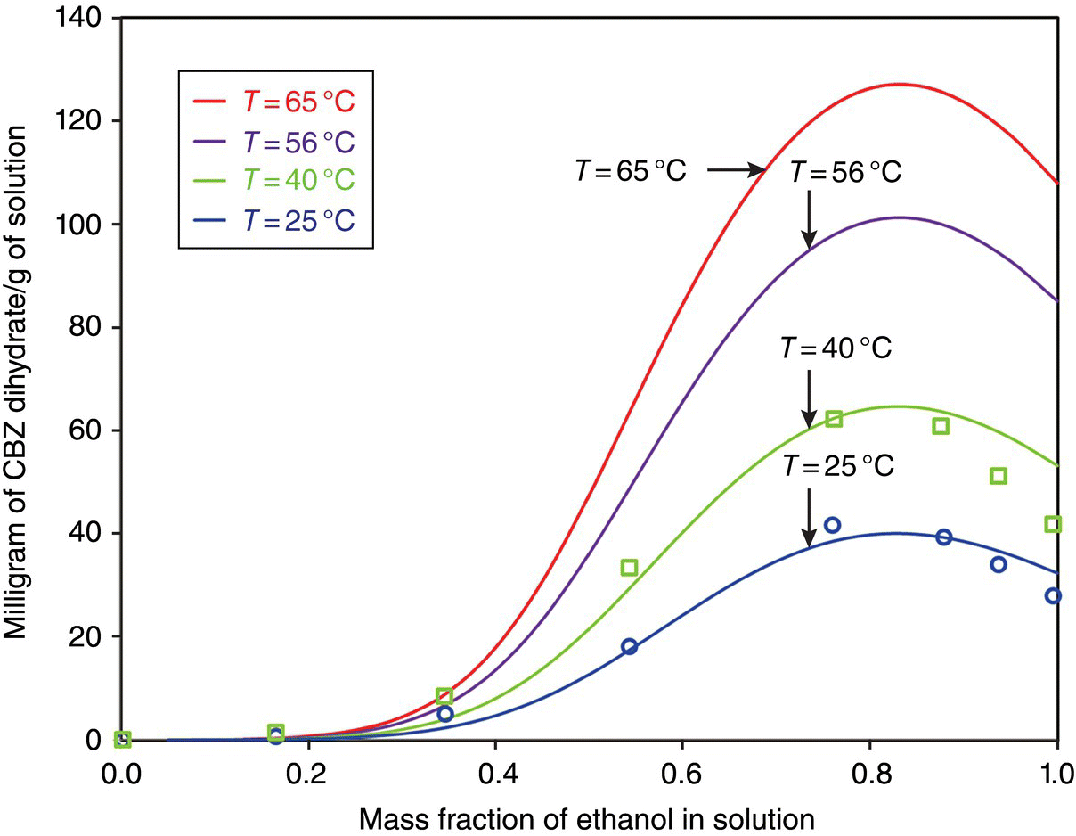
FIGURE 26.5 Solubility of carbamazepine dihydrate as a function of mass fraction of ethanol (solvent) at different temperatures. Solid curves are predictions from NRTL‐SAC model, while the open symbols are the experimental data points.
The conceptual segment contribution approach in NRTL‐SAC represents a practical alternative to the UNIFAC functional group contribution approach where extension to solvents with different functional groups may not be reliable [5]. This approach is suitable for use in the desired industrial practice of carrying out measurements for a few selected solvents and then using NRTL‐SAC to quickly predict other solvents or solvent mixtures and to generate a list of suitable solvent systems. In this case, the NRTL‐SAC model not only helped in solvent selection but, in conjunction with DynoChem® models for the antisolvent and cooling crystallizations, also enabled crystallization process optimization and scale‐up.
26.3 ESTIMATION OF NUCLEATION AND GROWTH KINETICS
With a rigorous understanding of equilibrium solubility, another important insight into crystallization process design is afforded by exploring nucleation and growth kinetics. Estimation of nucleation and growth kinetics requires mathematical description of the evolution of the crystallization process, the framework for which is an appropriate population balance model (PBM). The PBM describes the dynamic evolution of the crystal size distribution (CSD) as a result of various governing processes including nucleation, growth, aggregation/agglomeration, and breakage. These processes are also governed by the supersaturation and hence the concentration profiles. The relationships between these various processes are schematically represented by Figure 26.6. Reaction, resulting in the generation/depletion of a species and/or the amount of material initially present in a crystallization system, determines the liquid‐phase concentration. Concentration, along with the temperature and/or solvent composition, leads to supersaturation, which induces nucleation, growth, and potentially particle aggregation/agglomeration. Growth affects concentration and the product CSD. Nucleation as well as aggregation/agglomeration also affects the resultant CSD, but their impact is oftentimes influenced by the system hydrodynamics and interactions between various solid interfaces. Hydrodynamics and solid–solid interactions often affect the extent of crystal breakage/attrition due to shear and impact, which also controls the product CSD. Boundary conditions for the solution of a PBM are described by initial concentration, solvent composition, temperature, and the seed CSD where appropriate.
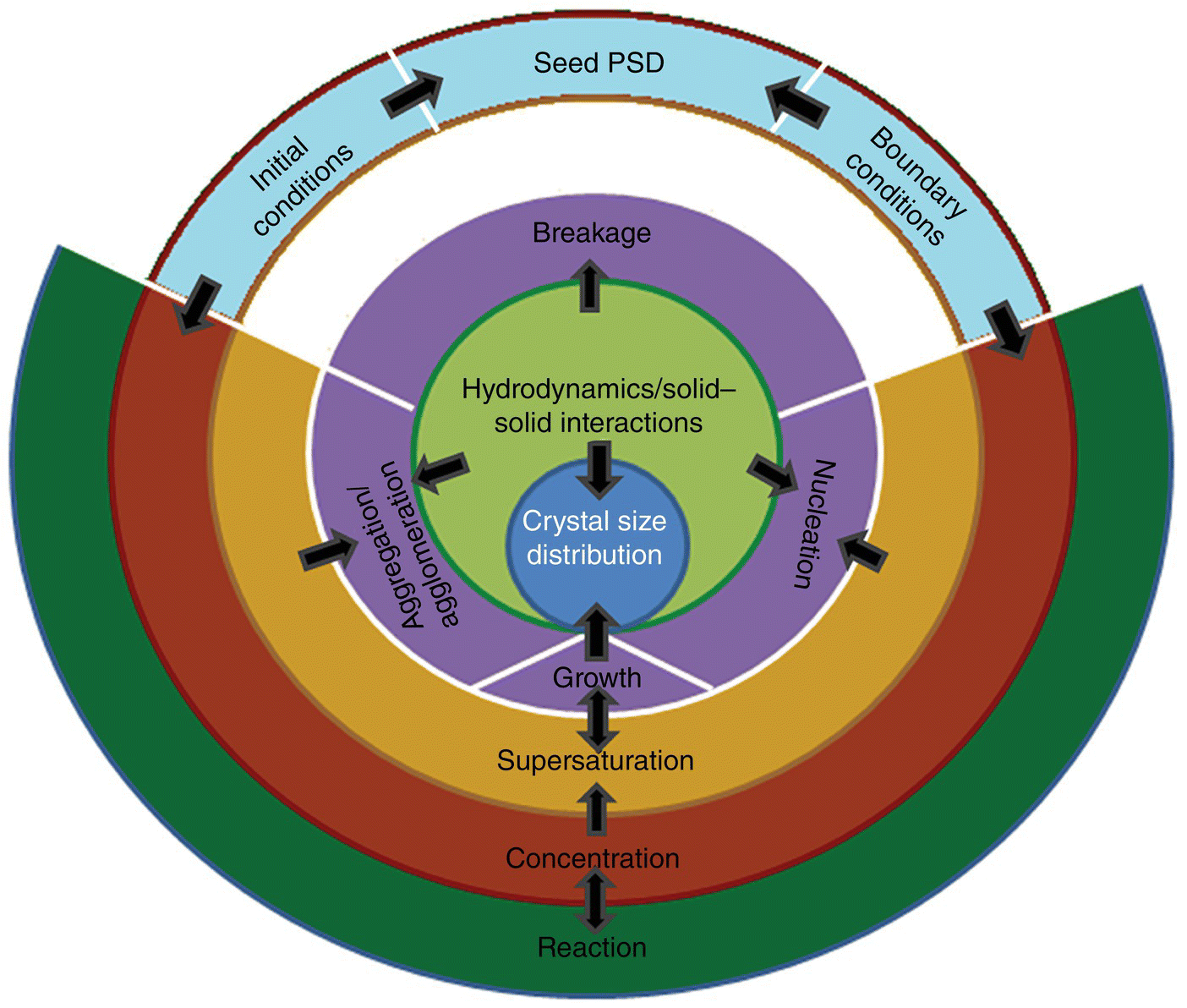
FIGURE 26.6 Interplay between various underlying processes that impact the crystallization process and resultant crystal size distribution.
Thus there exists a complex interplay between various underlying processes, and its quantification can be of significant use in the holistic design of crystallization processes. However, this section will focus on the methodologies to estimate only nucleation and growth kinetics for the sake brevity.
26.3.1 Forward and Inverse Problem Approach‐based Methodologies
Most of the methods reported in the literature to estimate the kinetics of crystal nucleation and growth can be broadly classified as using either a forward problem or inverse problem approach. A schematic depicting the essence of these two approaches to model extraction is shown in Figure 26.7. The forward problem approach shown in Figure 26.7a is based on a starting point of a presumed form of the model with correct inputs, parameter settings, initial and boundary conditions, etc., which is used to arrive at the final solution (CSD). Using this approach, the kinetics of primary nucleation is oftentimes extracted using MSZW estimation and induction time measurements. Growth kinetics are estimated by regressing its parameters so as to yield a better fit of the experimental data with the predictions due to PBM in conjunction with the concentration profiles. This approach is predicated on an a priori assumption of a particular form of growth kinetics, with unknown parameters yielded as an output of the regression exercise.
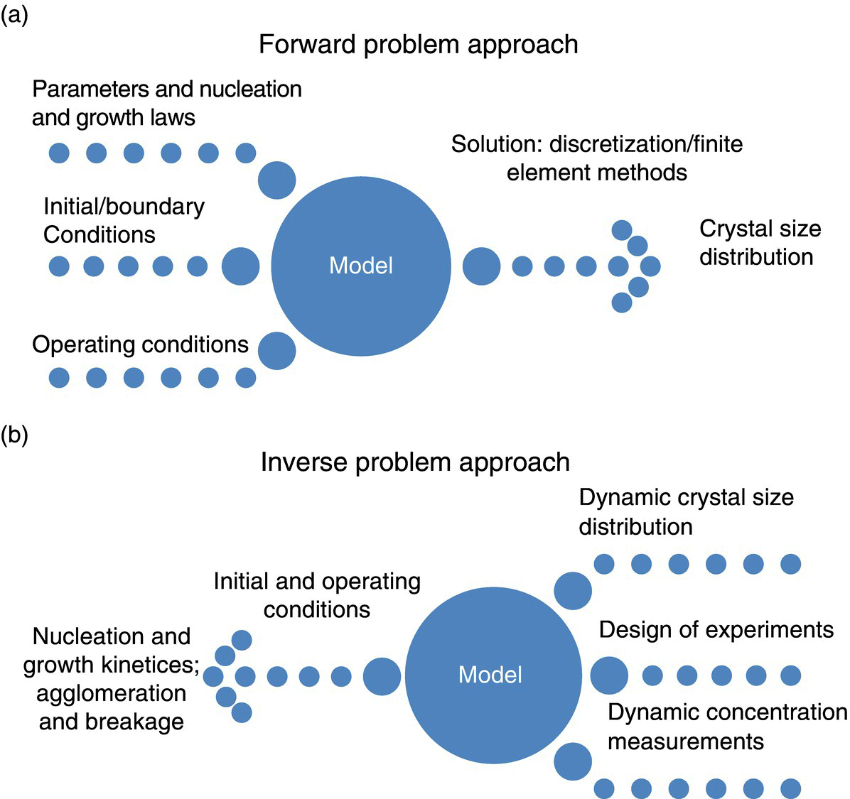
FIGURE 26.7 Schematic representing the forward (a) and inverse (b) problem approaches to estimate nucleation and growth kinetics.
In the absence of known nucleation kinetics, one can also resort to regressing its parameters along the lines of growth kinetics estimation.
The inverse approach relies on starting with the solution (CSD derived from experimental data) to determine what an appropriate model is for estimating nucleation and growth rates. This approach relies on mathematical analysis of PBM and dynamic data on CSD and concentration obtained from the careful design of experiments. This approach, unlike the forward problem approach, is independent of any assumption regarding the form of the nucleation or growth models. Although obviously powerful, this approach is rarely used in industrial practice, seemingly due to the perceived complexity of the methodology. However, the power of this approach warrants further advancements and simplifications in order to promote industrial use.
Most practical approaches today are based on the simplifying assumption of having a spatially and temporally homogeneous particulate system, which is characterized by a single particle dimension. However, the convergence of highly efficient computational methodologies and novel technologies to characterize three‐dimensional crystal size and shape distributions holds promise for reducing such simplifying assumptions in the future.
26.3.2 Case Studies for Estimation of Nucleation and Growth Kinetics
Three case studies employing some of the popular methodologies to estimate nucleation and growth kinetics are discussed in this section, each showcasing details regarding the approach and its implementation. The first case sheds light onto the inverse PBM approach‐based technique, reported by Mahoney et al. [7]. It is then followed by an example in which the approach was used to estimate particle growth rates to inform the selection of appropriate cooling rate to support process scale‐up. The second case study, based on the work presented by Mitchell and Frawley [8], illustrates the approach of induction time measurement via in situ techniques to estimate the nucleation kinetics. The final case study describes how the data obtained from experiments involving supersaturation spikes were used to determine nucleation and growth kinetics for both a cooling and an antisolvent crystallization. Taken together, this work provides practical theory coupled with industrially relevant case studies, providing an overview of options for interrogating nucleation and growth kinetics.
26.3.2.1 Case Study 1: Inverse Problem Approach to Extract Crystallization Kinetics
This section elaborates on the inverse problem approach to extract crystallization kinetics, details of which have been reported in the literature [7]. Application of a part of this methodology has been then illustrated through the case of CBZ dihydrate crystallization.
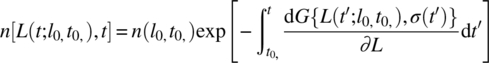
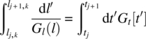
The population balance equation (PBE) describing the number density of the crystals (defined as the number of crystals per unit of “size” measure per unit volume in the crystallizers) involving only nucleation and growth can also be written as
with the boundary condition described by

where
- n(L, t) is the number density of the crystals with the internal coordinate of crystal size, L.
- G[L, σ(t)] is the growth rate that depends on both the size, L, and the supersaturation, σ.
- B is the nucleation rate.
Note that the supersaturation can also be expressed in terms of time, t, to get a simple algebraic expression for subsequent numerical treatment.
In this approach, the PBE is solved by the method of characteristics under the suitable assumptions of the deterministic growth rate and no or minimal aggregation/breakage. This associates the population of crystals of any size at any time with a single point from the initial (i.e. existing crystals from seeding) or boundary condition (i.e. nucleation). The key to leveraging this approach is the recognition that these growth characteristics correspond to the size history of individual crystals and that they can be linked with the fixed cumulative number of the crystals. These growth characteristics are directly identified from the experimental time measurement of crystal size or chord length distributions. The variability in the size for a given set of cumulative oversize number (CON) (counts) along these characteristics provides decoupled equations that can be used to determine the growth rate.
The solution to the PBE along these growth characteristics is given by
For no aggregation, the crystal number density depends only on the characteristic passing through the initial size. The key idea is that the characteristics can be readily determined from the data on the CSD as a function of time by identifying that there is no influence from the nuclei to the population of larger particles. Quantiles refer to the locus of constant numbers over a size cut. The cut indicative of size must move as the characteristic. Under suitable assumptions of deterministic growth and known (or absent) aggregation, characteristics correspond to a constant number oversize.
Figure 26.8 shows how the method of characteristics is used to construct the solution to the PBE.
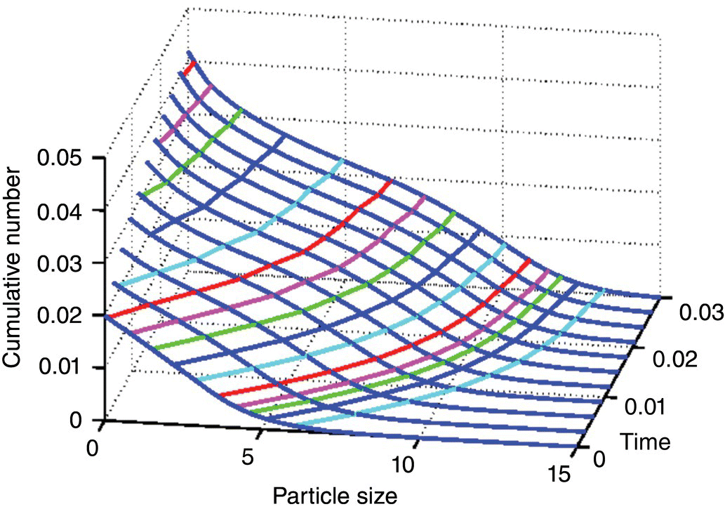
FIGURE 26.8 Plot of cumulative oversize number as a function of particle size for various times.
The solution in terms of the number density along the characteristic curves of the first‐order partial differential equation follows individual particle growth paths. One can readily envision that the number density can change due to growth and aggregation. The paths are solely dependent on particle growth. Thus, the characteristic curves show how the single particles develop from their initial sizes. Furthermore, they directly relate to both growth of nuclei and initial crystals. Each of the constant CON, defined as the total number of crystals with the size larger than a given size under consideration, lines would intersect the CON time profiles, and the projections of these intersections on the particle size coordinate would yield a size vs. time trajectory. These trajectories are nothing but the growth characteristics and are depicted in Figure 26.9.
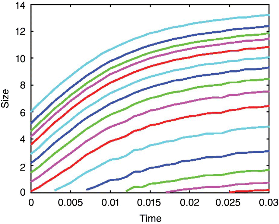
FIGURE 26.9 Growth characteristics extracted from Figure 26.8.
The crystal growth characteristics in the plot shown in Figure 26.9 are represented by Eq. (26.15):
The following subsection describes the estimation of growth and nucleation kinetics in further detail.
26.3.2.1.1 Kinetics of Crystal Growth
The assumption of treating the growth rate expression as a degenerate function of size‐ and supersaturation‐dependent components makes the determination of the growth kinetics in more of a complete sense. The product of the crystal number density and the size dependent part of the growth expression can be readily shown to be an exact invariant along the growth characteristic. Thus one may solve the characteristic equation as above (Eq. 26.15) and notice that the right‐hand side is independent of the quantile, while the left‐hand side depends on it. For each quantile one can calculate the right‐hand side and examine if the calculations coincide. Thus for a separable growth law (i.e. degenerate form), we have
The variation of the number density along the characteristics is used with the conserved quantity to provide the system of equations where Nq is the total number of quantiles tracked. Thus along the growth characteristics, we have nj, kGl(lj, k) = nj + 1, kGl(lj + 1, k) where k takes value from 1 to Nq. The growth law can be expanded in terms of the appropriate basis functions to form residues, which can be minimized to obtain the size‐dependent growth law. The advantage of this approach is that one can select the basis functions informed by assumed or known growth mechanisms. The expansion in trial basis functions permits the extrapolation of the characteristics to their origin either on the time axis (for nuclei) or to the size axis (initial particles). Local Hermite cubic basis functions could be used in the absence of the known growth forms as it takes care of the fact that different mechanisms may dominate in different size regions. The time‐dependent or the supersaturation‐dependent growth law can easily be extracted using the following equality for the residue formation and subsequent error minimization:
Thus the overall growth law presumed to be a degenerate function as discussed on the onset of the discussion can be completely determined as a function of both the supersaturation and size.
26.3.2.1.2 Kinetics of Nucleation
Once the growth law is completely determined, then one can make use of the fact that the measured CSD evolution over time from each experiment arises from the initial and boundary conditions according to the solution of the PBE along the characteristics. Each measurement can be traced back to either the initial or boundary condition using the determined growth law. The collapse of these measurements onto the same master curve is equivalent to the prediction of the data, and the dispersion of the collapse is due to experimental or model error. This allows a verification of the model assumptions, i.e. deterministic separable growth law, and also gives the initial and boundary conditions more accurately than using the experimental data nearest to those conditions. These conditions can be used subsequently in the determination of nucleation law.
While the reader is referred to the paper by Mahoney et al. [7] for full details, a practical protocol to extract the growth and nucleation kinetics is presented below.
26.3.2.1.3 Overall Protocol for the Kinetic Model Extraction
Below is a protocol to estimate nucleation and growth rates using the inverse problem approach.
- Experimental protocol:
- Determine the phase diagram for the crystallization of the compound of interest using guidance from Section 26.2 on solubility measurements.
- Estimate the temperature and/or solvent composition profile that will keep the crystallization system in a metastable region throughout the process so that nucleation can be controlled to promote growth rate. Reduced nucleation will lead to reduced aggregation, thus enabling the growth rate to be determined with better confidence.
- Carry out measurement of chord length distribution (CLD) using FBRM® technique with the optimal optical settings and physical position. Check the consistency of the total FBRM® count for different concentrations of crystals to ensure appropriateness of measurements. Ideally, the depth of FBRM® laser penetration and measurement zone should remain constant to keep the observable volume constant to the extent possible.
- Carry out the measurement of concentration as a function of time using ATR‐FTIR, online LC, or off‐line analysis of mother liquors obtained from the immediate filtration of slurry samples at appropriate temperatures.
- Preprocessing of the Lasentec® FBRM® data:
- Carry out the baseline correction by simply subtracting the data corresponding to the clear solution from the rest of the data. Replace negative counts (if any) by interpolated values corresponding to adjacent size channels.
- Smooth the data to eliminate abnormal fluctuations. Abnormality can be discerned based on knowledge/observation of the physical behavior that may be exhibited by the process. Check for the conservation of counts and the trend shown by total counts.
- Eliminate the outliers. This can be done by observing the evolution of the profile in the time coordinate.
- Conversion of the CLD measured by Lasentec® FBRM® to CSD:
- The CLD can be either directly used as is (the growth rate will correspond to the chord length) or transformed into CSD using various algorithms [9–12] of varying complexity available in commercial software (e.g. DynoChem®).
- It is advisable to verify the conversion of CLD to CSD to have meaningful data analysis and further interpretations. The CLD can be used as a direct measure to assess the crystallization performance if the relationship between the chord length and the target crystal size attribute can be established.
- Data processing to extract nucleation and growth kinetics using the inverse population balance approach:
- Discretize the time and size domain for CSD measurements done using an off‐line analysis method. For in‐line measurement, such as FBRM®, one can use appropriately spaced time points to reduce the burden on the amount of data to be processed. Data filtering should be done so as not to affect the extracted kinetics.
- Plot cumulative number count data.
- Extract crystal growth characteristics at various CONs.
- Select basis functions, and form a matrix equation for inversion to get the size‐dependent growth and then the supersaturation (which changes as a function of time due to progression of crystallization) growth, followed by the determination of the nucleation rate.
- Carry out the forward simulation using the extracted growth and nucleation rates to check with the measured evolution of CLD or CSD.
- Fit the discrete model form obtained from the inverse problem approach to a continuous one, assuming some kind of “well‐defined model” with accurate parameters.
- Carry out another experiment within the operating range, and measure the CSD/CLD time evolution along with the concentration measurements, and verify the same using the forward simulation with the extracted models following the earlier steps.
While the abovementioned exhaustive protocol could be followed for the complete determination of growth and nucleation kinetics, the following subsection illustrates an example of quick growth rate estimation.
26.3.2.1.4 Example Application of Inverse Problem Approach for Growth Rate Estimation
The following example shows how the inverse problem approach was used to assess the impact of cooling rate on crystal growth rates for a cooling crystallization of CBZ dihydrate from an ethanol–water solution. The information gained regarding growth rates from this exercise was used to optimize a linear cooling profile (parabolic cooling was not accessible with available equipment) to improve product physical properties under constrained project timelines.
A cooling crystallization was designed based on the solubility data generated in Section 26.2.5.4, the objective of which was to produce larger and thicker CBZ dihydrate crystals. Experiments (10 g scale) were performed at three different cooling rates (6, 2, and 1 °C/h) in an effort to identify the appropriate cooling rate to achieve desired crystal growth. While reduced cooling rates would be expected to favor growth, reduction beyond what is required to achieve the objective needlessly lengthens process cycle time and is therefore undesirable. In each experiment, a seed slurry (generated using a high‐shear wet mill) was added to a supersaturated solution at 48 °C, and the crystallization mixture was cooled down to 22 °C at the prescribed rate. Each experiment was monitored using Lasentec® FBRM to track the CLD over time. CLD data collected from the 1 °C/h experiment at discrete time points over the course of the crystallization is shown as an example in Figure 26.10. While the shape of the distribution is very consistent throughout the experiment, the evolution of the profile suggests growth over time. In this case, the chord length measurements were found to correlate with and be representative of the CSD, as confirmed by photomicrographs taken by laser microscopy.
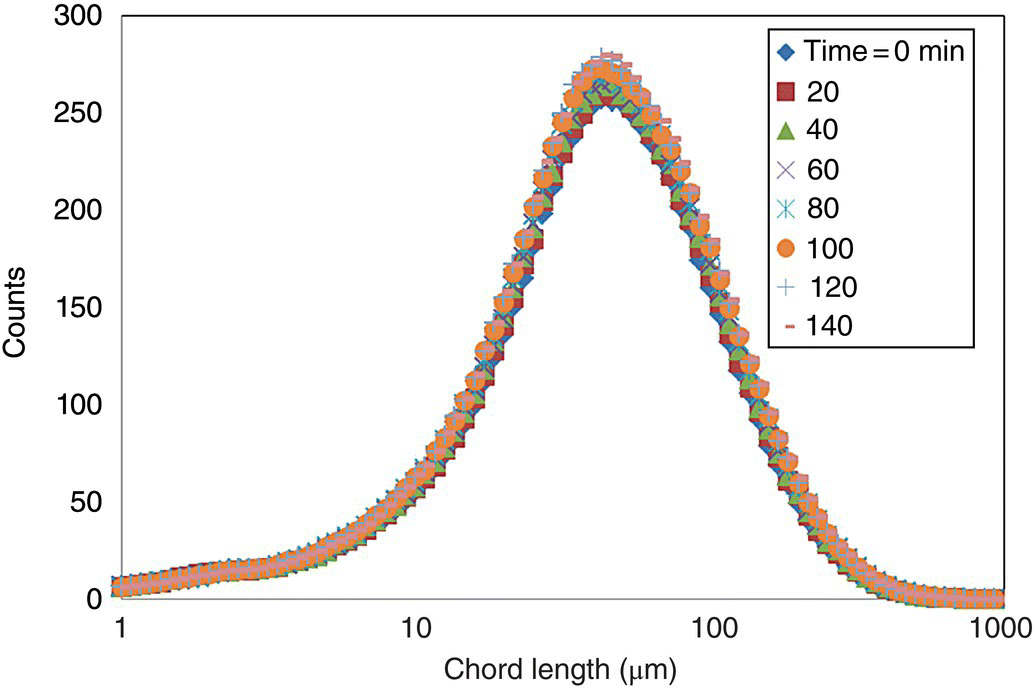
FIGURE 26.10 Raw FBRM data from the experiments carried out at the cooling rates of 1 °C/h.
The FBRM® data were then converted to CON profiles as a function of chord length. This analysis was performed on selected time points to simplify the extraction of growth characteristics in the next step. An example of the CON profile for the experiment using a cooling rate of 1 °C/h is shown in Figure 26.11.
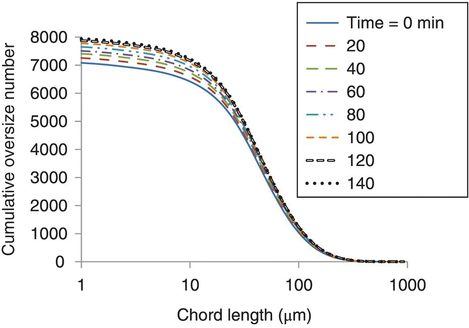
FIGURE 26.11 Cumulative oversize number as a function of chord length for selected time points for the cooling rate of 1 °C/h. Results presented as smoothed lines to improve readability.
The growth characteristics were then extracted for each experiment, as described previously, and shown in Figure 26.12. Equations describing the change in chord length over time are displayed for three selected crystal sizes (chord length at t = 0) for each experiment. The low chord length numbers in the 6 °C/h (Figure 26.12a) experiment compared with that of either the 2 or 1 °C/h experiments (Figure 26.12b and c, respectively) may be a manifestation of a greater extent of secondary nucleation occurring with increased cooling rates. Moreover, the growth trajectory associated with faster cooling experiments is enhanced compared with slower cooling experiments.
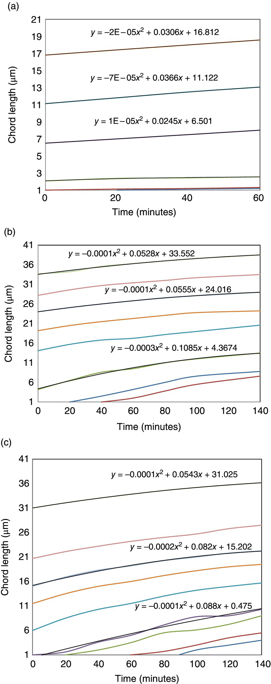
FIGURE 26.12 Growth characteristics extracted from the cumulative oversize plots (a) 6 °C/h, (b) 2 °C/h, and (c) 1 °C/h. Results presented as smoothed lines to improve readability.
The growth characteristics were then used to extract growth rates for various initial crystal sizes (indicated by the intercept on the y‐axis of Figure 26.12) at selected time points. A plot of the growth rate corresponding to initial crystal size for the cooling rate of 1 °C/h is shown in Figure 26.13 as an example.
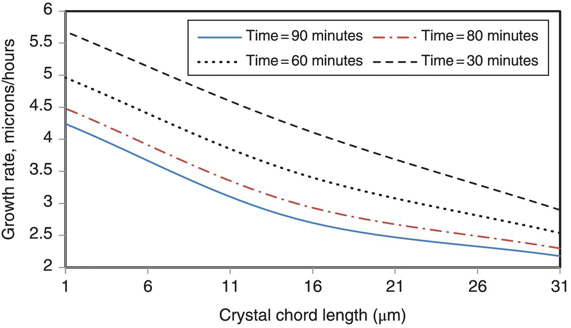
FIGURE 26.13 Growth rates extracted from the characteristics as a function of the crystal size represented as the chord length for selected time instances. Results presented as smoothed lines to improve readability.
Figure 26.13 shows that the growth rate is a function of the crystal size. Even though the objective of this study was not to interrogate the details of the growth kinetics, it is possible to de‐convolute the growth rate in terms of size‐dependent part and the time‐dependent (or corresponding supersaturation) part in accordance with the previously described procedure.
The average growth rate for each experiment was obtained by estimating growth rates for various sizes at discrete time points. In each case, time intervals were selected appropriately to enable observable growth over the suitable time window as permitted by the cooling rate. Table 26.2 lists the growth estimation time points used along with the average growth rates estimated for each experiment.
TABLE 26.2 Average Growth Rates for Various Cooling Rates
| Cooling Rate (°C/h) | Growth Estimation Time Points (min) | Average Growth Rate (μm/h) |
| 6 | 5, 10, 15 | 1.802 |
| 2 | 15, 30, 45 | 3.336 |
| 1 | 30, 60, 90 | 3.660 |
The data in Table 26.2 shows the expected trend such that the growth rate increases as the rate of cooling decreases. While there is a significant increase in growth rate from 6 to 2 °C/h, the increase in growth rate from 2 to 1 °C/h is only marginal. Based on this finding, the cooling rate implemented in the 15 kg pilot‐scale run was 2 °C/h. This allowed the processing to complete in the available manufacturing time with the assurance that sufficient growth of the crystal population would not be significantly compromised. The process scale‐up delivered product with the desired physical properties. The photomicrographs of the crystals obtained from the pilot‐scale run (2 °C/h) compared with the laboratory experiment, which was cooled at 6 °C/h, are shown in Figure 26.14a and b, respectively. The crystals using the slower cooling profile were both larger in size and exhibit a reduced, more favorable aspect ratio, as evidenced by the more platelike morphology of crystals shown in Figure 26.14a.
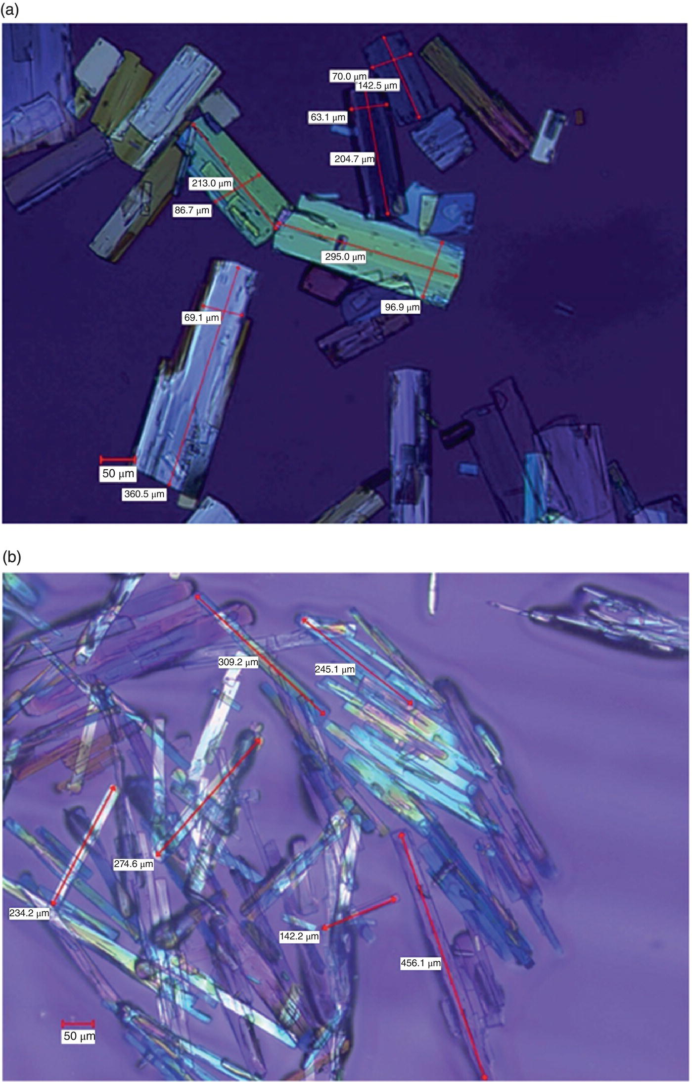
FIGURE 26.14 Photomicrographs of crystals resulting from the cooling rate of (a) 2 °C/h from the pilot plant and (b) 6 °C/h from laboratory experiment.
In summary, the presented example shows that an inverse population balance approach is useful for estimating crystal growth rates without the need to rely on complex calculations. This approach was enabled in a timely fashion by three simple lab‐scale experiments and appropriate treatment of CLD data. These data provided the basis to incorporate a timesaving optimization of the crystallization process while minimizing risk to product quality.
26.3.2.2 Case Study 2: Measurement of Nucleation Rate From Induction Time Measurement
In this example reported by Mitchell and Frawley, nucleation kinetics were estimated based on induction time via measurement of the MSZW [8, 13, 14]. Estimations of nucleation kinetics were presented in this work using two theoretical approaches: (i) classical nucleation theory reported by Nyvlt [15] and (ii) a modification of the Nyvlt approach in which MSZW is assumed to be dependent upon the technique used to detect particle formation as reported by Kubota [16].
The MSZW is defined as the gap between thermodynamic solubility and the supersolubility required for solid particles to form. The schematic shown in Figure 26.15 shows the solubility and supersolubility plotted as a function of concentration and temperature; at any given concentration, the temperature gap between these curves is defined as the MSZW.
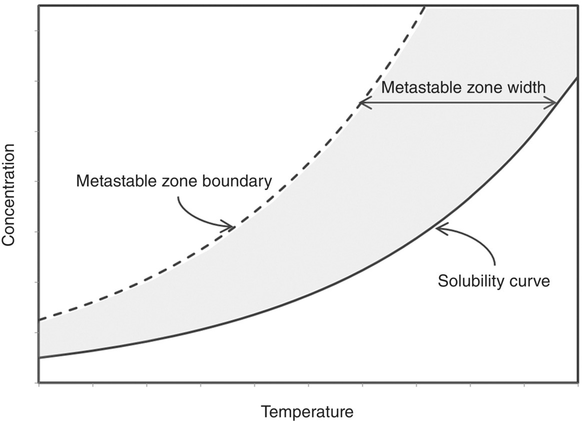
FIGURE 26.15 Schematic showing typical solubility and metastable zone width boundary curves in relation to the metastable zone width (MSZW).
Based on classical nucleation theory and appropriate assumptions, the cooling rate, R, can be expressed in terms of the MSZW (expressed as ∆Tmax), the apparent nucleation order, m, the nucleation rate constant, kn, and the thermodynamic solubility concentration, c*, as shown in Eq. (26.18):
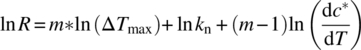
Using this approach put forth by Nyvlt, the log/log plot of cooling rate vs. MSZW yields a straight line with a slope commensurate with the apparent nucleation order (m) and kn estimated from the y‐intercept.
Kubota’s modification of classical nucleation theory expresses the nucleation rate in terms of the number density (Nm/V) and the true nucleation order (n) as shown in Eq. (26.19). This enables estimation of a number‐based nucleation rate rather than the mass‐based nucleation rate afforded by Nyvlt’s approach:
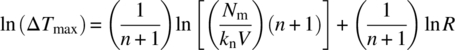
Equation (26.19) can be readily rearranged, resulting in Eq. (26.20):
Thus, using Kubota’s approach, the nucleation order can be estimated from the slope of the line on a log/log plot of MSZW vs. cooling rate at a given saturation concentration. The nucleation rate constant, kn, can be extracted from the intercept with an assumed value of the detectable number density for the detection technique used. Table 26.3 summarizes the nucleation parameters estimated from each approach and how they are derived from measurement of the MSZW.
TABLE 26.3 Summary of Nucleation Parameters Estimated from Nyvlt and Kubota Approaches Along with Estimated Values for Paracetamol in Ethanol System Based on Induction Time Measurement
| Approach | Basis | Nucleation Order | Kinetic Nucleation Parameter |
| Nyvlt | Equation (26.18), Figure 26.17a | m, apparent nucleation order m = slope |
kn |
| Estimated value, paracetamol in ethanol | 1.68 ± 1.25 | 0.206 ± 0.13 | |
| Kubota | Equation (26.19), Figure 26.17b | n, true nucleation order n = slope − 1 |
|
| Estimated value, paracetamol in ethanol | 0.76 ± 0.66 | 191.7 ± 464.1 |
A significant benefit of the approach put forth by Kubota is that it establishes a relationship between MSZW and nucleation induction time. The induction time is described as the time required for the number density (Nm/V) to reach a fixed value. Assuming induction time can be described by a power law expression and the ∆T is constant (experiments are conducted isothermally), the induction time (tind) can be written as a function of the number density, nucleation constant, and the degree of supercooling as shown in Eq. (26.21):
Both the Nyvlt and Kubota approaches were applied to characterizing the nucleation of paracetamol in ethanol as described below. Figure 26.16 shows the cloud point of paracetamol/ethanol solutions as a function of concentration and temperature. Reported methodology involved rapidly cooling solutions to the desired temperature and then holding under isothermal conditions until nucleation was observed using a turbidity probe. The time between reaching the target supercooling and the detection of the first nucleation events was taken as the induction time for the nucleation process. The MSZW was determined by comparison of saturation conditions (literature reported values) and the measured cloud point. These data show that the MSZW (horizontal distance between supersolubility data and solubility curve) increases with increasing saturation temperature. Moreover, comparison of data collected at cooling rates at 0.5 and 1 °C/min (as well as 0.2 and 0.7 °C/min, data not shown) suggests that the measured MSZW is wider using faster cooling rates.
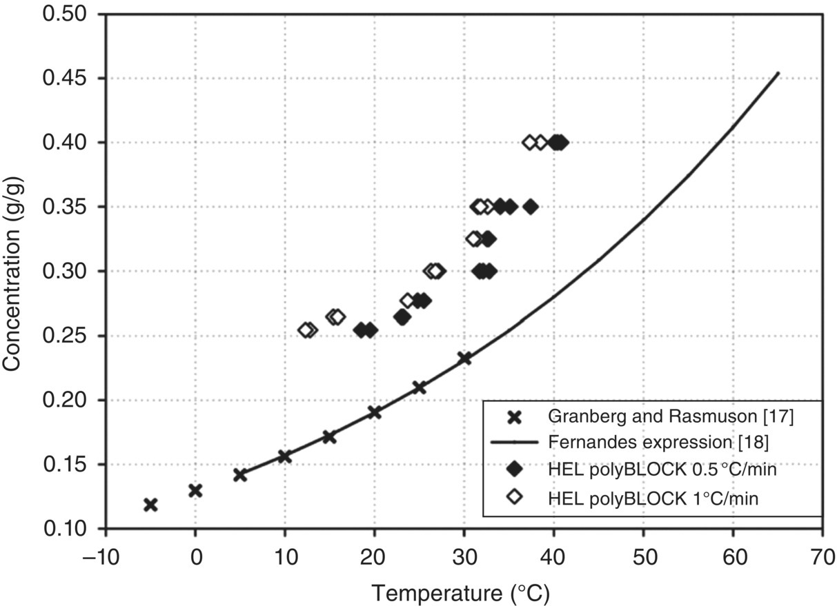
FIGURE 26.16 Measure cloud point for cooling rates of 0.5 and 1 °C/min along with the literature solubility data for paracetamol in ethanol.
It is also reported in this work that the MSZW decreases slightly with an increase in mixing intensity. Hence, it is recommended to keep mixing intensities during the measurement of MSZW similar to those to be used in the anticipated crystallization process to mitigate this effect.
Based on this data, nucleation kinetic parameters were estimated using both Nyvlt and Kubota’s approaches using Eqs. (26.18) and (26.20), respectively. Figure 26.17a shows log/log plots of cooling rate vs. MSZW derived from the Nyvlt approach, and Figure 26.17b shows log/log plot of MSZW vs. cooling rate arrived at from the Kubota approach. The nucleation parameters estimated using both approaches are summarized in Table 26.3. It is notable that using Kubota’s approach, kn can be evaluated by assuming a value of the detectable nuclei size of the cloud point detection technique used; a detectable nuclei size of 10 μm was used.

FIGURE 26.17 Nucleation order estimated from MSZW data for a saturation temperature of 44 °C using (a) Nyvlt approach derived from classical nucleation theory and (b) Kubota‐modified approach that corrects for the limit of detection of the turbidity measurement.
The absolute values of the constants differ significantly, and this results in a difference in the estimated nucleation rates. A plot of the nucleation rate vs. supersaturation estimated using both the Nyvlt and Kubota approaches is shown in Figure 26.18. This figure shows that the nucleation rate profile predicted using the Kubota approach is different from that obtained using the Nyvlt approach, with a crossover point between the two prediction curves.

FIGURE 26.18 Estimated nucleation rates as a function of supersaturation obtained using both the Nyvlt and Kubota approaches.
A key insight provided by the Kubota approach is the ability to predict nucleation induction time, which was demonstrated and confirmed experimentally in this work. Figure 26.19 shows the measured induction time at two saturation temperatures (30 and 40 °C) vs. the degree of supercooling compared with the predictions using the Kubota approach. The experimental data are in close agreement with theoretical predictions.
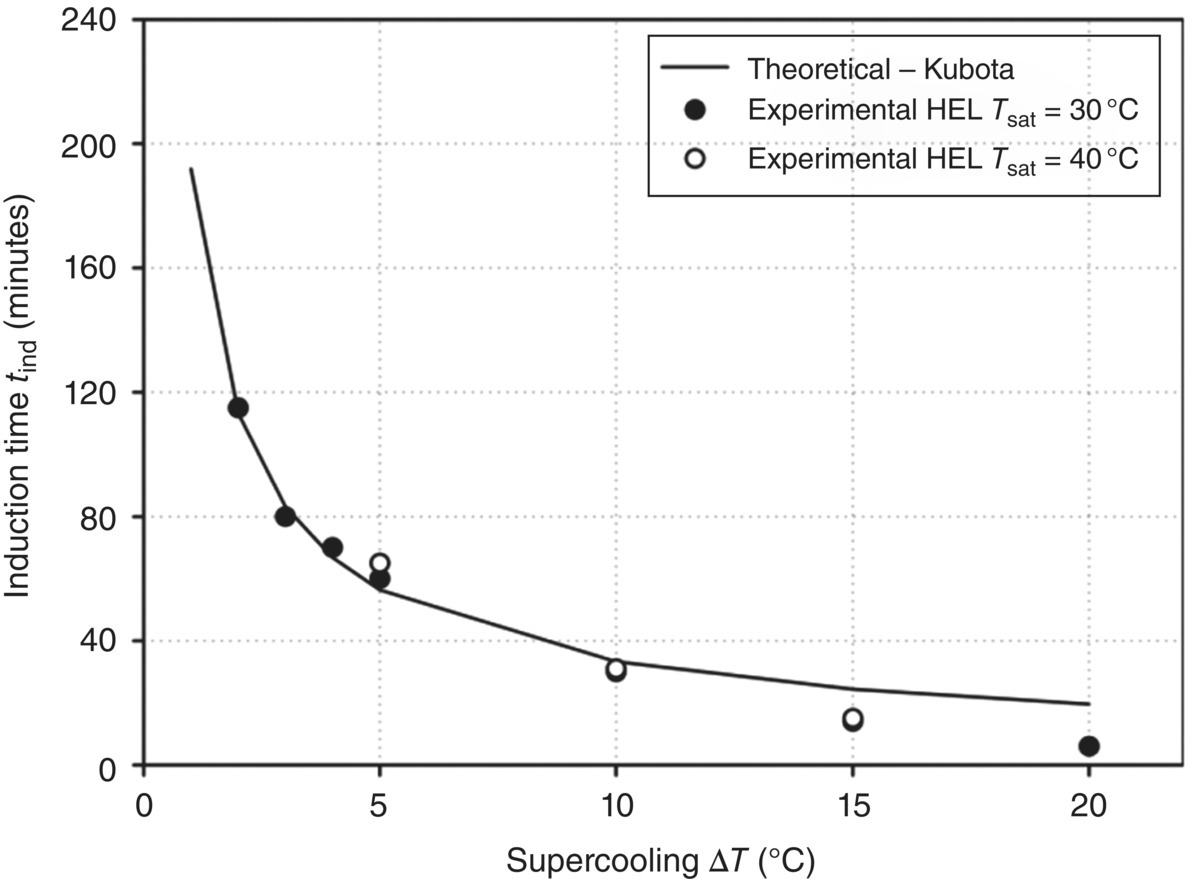
FIGURE 26.19 Experimentally measured induction time as a function of supercooling for paracetamol in ethanol mixtures vs. predicted induction times using Kubota’s approach.
In summary, the work of Mitchell and Frawley demonstrates how the measurement of MSZW can be used to estimate nucleation kinetic parameters using the approach of Nyvlt (based on classical nucleation theory) and Kubota’s modified approach. Kubota’s approach affords key advantages that include (i) the estimation of a number‐based nucleation rate, for which the limit of detection for the cloud point determination technique factors into the calculation, and (ii) ability to relate the MSZW to the nucleation induction time for a given system. The measured induction time for the paracetamol–ethanol system studied showed close agreement with induction times predicted using Kubota’s approach across the range of supersaturations evaluated. While this example demonstrates estimation of nucleation kinetics for a cooling crystallization, an analogous approach can be applied to an antisolvent crystallization; the reader is directed to the work published by authors on paracetamol in methanol–water antisolvent crystallizations for further information.
26.3.2.3 Case Study 3: Estimation of Nucleation and Growth Kinetics for Cooling and Antisolvent Crystallizations Using Supersaturation Spikes
26.3.2.3.1 Introduction
Understanding of nucleation and growth kinetics can be an important consideration when first evaluating different modes of crystallization for a given system. In this example, crystallization kinetics extracted from the forward problem approach were studied for a particular drug substance of interest to inform whether a cooling crystallization process or antisolvent addition process would produce the desired drug substance properties. The crystallization process can be described by alternate form of PBE.
Let us put conventional PBE for size‐independent growth rate here that is used to derive moment equations:
The change in solute concentration solely due to growth of the seed crystals can be described by Eq. (26.23), where kv, ρc, G, and n are the volumetric shape factor, crystal density, growth rate, and population density of crystals, respectively:
The expressions describing the nucleation or birth rate (B) and growth rate (G) as a function of supersaturation (S) are shown in Eqs. (26.24) and (26.25). Hence, four parameters, kb, b, kg, and g, are required to describe the crystallization kinetics using this model:
The simple experiments performed to obtain the data needed to regress these crystallization parameters involve generating spikes of supersaturation within the crystallization system and then monitoring particle properties and drug substance concentration over an isothermal/isocratic hold period at these conditions. As described below, analysis of data from these experiments can provide valuable insight into crystallization kinetics that can inform the crystallization development process.
The methodology is predicated on the moment equations derived from PBE. For size‐independent growth rate, the PBE for the system accounting for only nucleation and growth reduces to the following general equation for jth moment:
where
- L0 is the size of detectable nuclei.
26.3.2.3.2 Experimental Description
In these studies, supersaturation was created by either decreasing temperature or adding antisolvent into the crystallization mixture. During the hold period after the spike, the CLD (using Lasentec® FBRM®) and drug substance concentration (using HPLC and mid‐IR) were monitored over time until complete de‐supersaturation (or saturation) was achieved. In the case of the cooling crystallization, drug substance was dissolved in ethanol at a higher temperature. Then the first temperature spike was generated at 45 °C and subsequently reduced stepwise to 40, 35, 25, and 5 °C. In the case of the antisolvent addition crystallization, water was added to an ethanol solution of drug substance in incremental spikes, making the weight percent water in the crystallization range from 34 to 59%. Using the CLD data and concentration profiles, crystallization kinetic parameters for simple nucleation/growth models were regressed. As the most reliable data are collected in the first spike (when a supersaturated solution is seeded), the exponents b and g are regressed for only that step and are subsequently fixed for the remaining spikes; only kb and kg are regressed from the data collected from remaining spikes. In this case, values for b and g were obtained from four parameter regressions of the data from 45 °C temperature spike (g = 1.789 and b = 2) and were fixed at these values for regression crystallization kinetic parameters for the remaining temperature‐induced and all antisolvent‐induced supersaturation spikes.
26.3.2.3.3 Results and Discussion
Figures 26.20 and 26.21 depict measured and regressed concentration as well as moments of CSD (μ0, μ1, μ2, and μ3) for a first (seeded) spike for the case of the cooling crystallization and antisolvent addition crystallization, respectively. In general, modeled results are in reasonable agreement with the experimental data extracted from CLDs (or assumed concentration profiles for the cooling case).

FIGURE 26.20 Modeled and measured concentration and CSD moment profiles (μ0, μ1, μ2, and μ3) at T = 45 °C for the cooling crystallization.
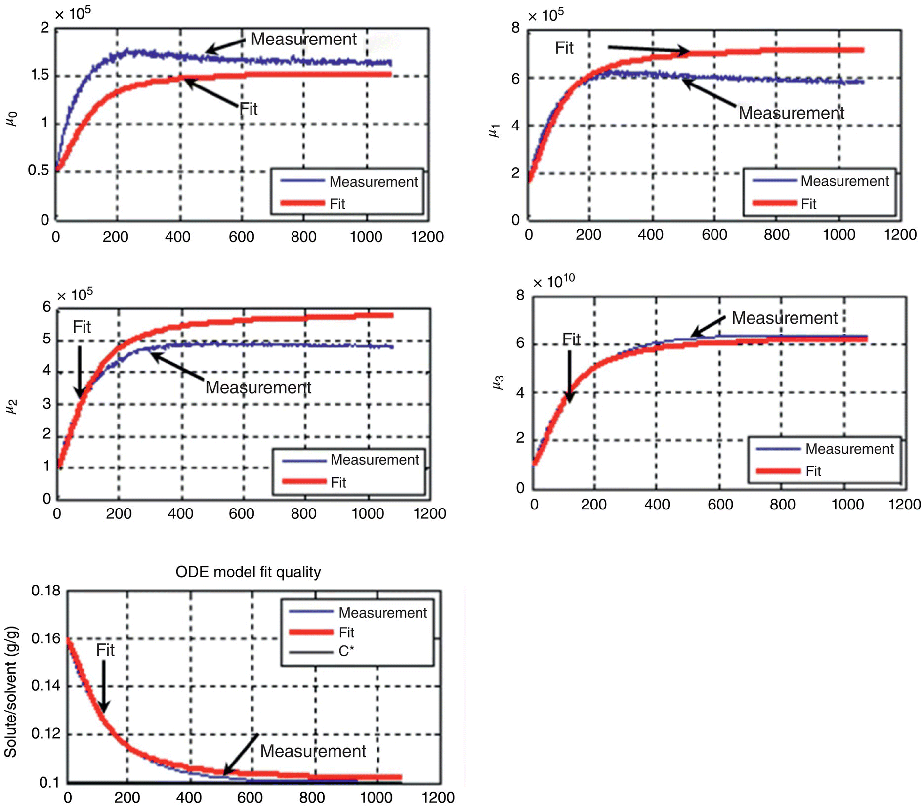
FIGURE 26.21 Modeled and measured concentration and PSD moment profiles of antisolvent crystallization at 34 wt % water and T =40 °C.
The results for the kinetic constants for both the cooling and the antisolvent crystallization processes, along with plots of kinetic parameters as a function of temperature or solvent composition, are summarized in Figure 26.22. Several insightful observations can be made regarding these data. First, Figure 26.22b shows that there is an exponential increase in kinetic parameters as temperature increases. Over the temperature operating range of 5–45 °C, kb and kg change by two orders of magnitude. The kinetic parameters, however, are much less sensitive to changes in solvent composition, wherein kb and kg change by two‐ to six fold over the crystallization operating range of 30–50 wt % water. The second notable point is that both growth and nucleation are more favored at higher temperatures and lower water content crystallization systems. Lastly, the ratio of kg to kb (which is a measure of the propensity to grow rather than to nucleate and tabulated in Figure 26.22a and c) is higher in the case of the antisolvent crystallization compared with the cooling crystallization.

FIGURE 26.22 (a) Estimated kinetic constants for supersaturation spikes of the drug substance cooling crystallization along with (b) corresponding plot of regressed kinetic parameters as a function of temperature. (c) Estimated kinetic constants for supersaturation spikes of the drug substance antisolvent crystallization along with (d) corresponding plot of regressed kinetic parameters as a function of weight percent water (antisolvent) in the crystallization system. Legend: squares, kb (nucleation) on the left axis; diamonds, kg (growth) on the right axis.
The above observations are indicative of the fact that an antisolvent crystallization design may be a better option for a robust, controllable, and scalable process dominated by crystal growth. Follow‐on experiments were performed to further interrogate this hypothesis. Crystals obtained from both the cooling crystallization and the antisolvent crystallization are shown in Figure 26.23. Crystals obtained from the cooling crystallization (Figure 26.23a) appear as a mixture of primary particles and agglomerates exhibiting a thin lath morphology. From the antisolvent crystallization (Figure 26.23b), thicker prismatic crystals were obtained, which proved to be more easily processable in the downstream isolation and drug product process.

FIGURE 26.23 Polarized light microscopy images of product from (a) cooling crystallization and (b) antisolvent addition crystallization.
The knowledge of crystallization kinetics and the MSZW was used to inform the appropriate antisolvent addition rate to sustain crystal growth throughout the crystallization. Furthermore, the seed loading was increased after initial pilot‐scale batches to minimize secondary nucleation upon scale‐up. This process, developed based on a solid foundation of nucleation and growth kinetics, has been successfully commercialized and shown to consistently deliver the appropriate DS physical properties.
26.4 SUMMARY
Fundamental understanding of solubility and nucleation/growth kinetics is the foundation upon which to develop and scale‐up robust, commercial‐ready crystallization processes. Solubility considerations, best practices, and example applications discussed herein provide insight into readily accessible means of enhancing understanding gleaned from these fundamental studies. Different approaches to understanding nucleation and growth kinetics are also presented and then discussed in the context of both literature examples and industrially relevant process development challenges. As demonstrated in this chapter, the meaningful impact that fundamental understanding can have on process development decisions and timelines is significant; the techniques and approaches discussed are appropriate for use in routine crystallization process development.
ACKNOWLEDGMENT
Authors would like to acknowledge experimental support from Bradley Greiner, Pankaj Shah, Onkar Manjrekar, and Carlos Orihuela and appreciate useful technical discussions with Shailendra Bordawekar, Samrat Mukherjee, and Ahmad Sheikh.
REFERENCES
- 1. Gamsjäger, H., Lorimer, J.W., Scharlin, P., and Shaw, D.G. (2008). Glossary of terms related to solubility: IUPAC goldbook. Pure Appl. Chem. 80 (2): 233–276.
- 2. Kawakami, K., Miyoshi, K., and Ida, Y. (2005). Impact of the amount of excess solids on apparent solubility. Pharm. Res. 22 (9): 1537–1543.
- 3. Mullin, J.W. (2001). Crystallization, 4e. Oxford: Elsevier Butterworth‐Heinemann.
- 4. Murdande, S.B., Pikal, M.J., Shanker, R.M., and Bogner, R.H. (2011). Aqueous solubility of crystalline and amorphous drugs: challenges in measurement. Pharm. Dev. Technol. 16 (3): 187–200.
- 5. ASPEN Properties, Version 8.4. Burlington, MA: Aspen Technology, Inc.
- 6. Liu, W., Dang, L., Black, S., and Wei, H. (2008). Solubility of carbamazepine (Form III) in different solvents from (275 to 343) K. J. Chem. Eng. Data 53 (9): 2204–2206.
- 7. Mahoney, A.W., Doyle, F.J., and Ramkrishna, D. (2002). Inverse problems in population balances: growth and nucleation from dynamic data. AIChE J. 48 (5): 981–990.
- 8. Mitchell, N.A. and Frawley, P.J. (2010). Nucleation kinetics of paracetamol‐ethanol solutions from metastable zone widths. J. Cryst. Growth 312: 2740–2746.
- 9. Tadayyon, A. and Rohani, B. (1996). Determination of particle size distribution by ParTec_100: modeling and experimental results. Part. Part. Syst. Charact. 15: 127.
- 10. Worlitschek, J. (2003). Monitoring, modeling and optimization of batch cooling crystallization. PhD Dissertation, Swiss Federal Institute of Technology, Zurich, Switzerland.
- 11. Li, M. and Wilkinson, D. (2005). Determination of non‐spherical particle size distribution from chord length measurements. Part 1: theoretical analysis. Chem. Eng. Sci. 60: 3251.
- 12. Nere, N.K., Ramkrishna, D., Parker, B.E. et al. (2006). Transformation of the chord length distributions to size distributions for non spherical particles with orientation bias. Ind. Eng. Chem. Res. 46: 3041–3047.
- 13. Mitchell, N.A., Ó’Ciardhá, C.T., and Frawley, P.J. (2011). Estimation of the growth kinetics for the cooling crystallization of paracetamol and ethanol solutions. J. Cryst. Growth 328: 39–49.
- 14. Ó’Ciardhá, C.T., Frawley, P.J., and Mitchell, N.A. (2011). Estimation of the nucleation kinetics for the anti‐solvent crystallization of paracetamol in methanol/water solutions. J. Cryst. Growth 328: 50–57.
- 15. Nyvlt, J. (1968). Kinetics of nucleation in solutions. J. Cryst. Growth 3–4: 377–383.
- 16. Kubota, N. (2008). A new interpretation of metastable zone widths measured for unseeded solutions. J. Cryst. Growth 310: 629–634.
- 17. Granberg, R.A., Rasmuson, A.C. (1999). Solubility of paracetamol in pure solvents. J. Chem. Eng. Data 44 (6): 1391–1395.
- 18. Fernandes, C. (1999). Effect of the nature of the solvent on the crystallization of paracetamol. Proceedings of the 14th International Symposium on Industrial Crystallization. Cambridge, UK.