
20
DRUG SOLUBILITY, REACTION THERMODYNAMICS, AND CO‐CRYSTAL SCREENING
Karin Wichmann and Christoph Loschen
COSMO logic GmbH & Co. KG, Leverkusen, Germany
Andreas Klamt
COSMO logic GmbH & Co. KG, Leverkusen, Germany and Institute of Physical and Theoretical Chemistry, University of Regensburg, Regensburg, Germany
20.1 INTRODUCTION
20.1.1 Methods for Compounds in Solution
There is a variety of computational methods for the treatment of compounds in solution. The scope of this chapter is not to give an overview of them, but to concentrate on applications of COSMO‐RS, a very efficient method for the a priori prediction of thermophysical data of liquids. COSMO‐RS combines unimolecular quantum chemical calculations that provide the necessary information for the evaluation of molecular interaction in the fluid phase, with a very fast and accurate statistical thermodynamic procedure. It has established itself as an alternative to structure‐based group contribution methods (GCMs) on the one hand and to force field‐based simulation methods on the other hand. Because of its special approach, COSMO‐RS is a generally applicable method for compounds in solution. It has been applied successfully in such diverse areas as solvent screening, partitioning behavior, liquid–liquid and vapor–liquid equilibria, and ADME property prediction and for such diverse compound types as drugs, pesticides, common organic compounds, halocarbons, and ionic liquids. COSMO‐RS is used in chemical, pharmaceutical, agrochemical, and petrochemical industry.
In this contribution, three application fields important in drug development and drug production will be considered: solubility prediction and prediction of free energy of reaction in solution and co‐crystal screening. Solubility prediction methods are important during the drug design and development process, because in the early drug design phase compounds are often only virtually considered by computational drug design methods or the synthesized amount of substance is insufficient for experiments. In both cases the only tools for the selection of promising drug candidates with adequate solubility are computational methods that predict the solubility with sufficient accuracy just from the chemical structure of the compound. A method requiring experimental data for solubility prediction is unfeasible in this situation, since such data will not be available.
Prediction of thermodynamic properties of compounds in solution is also important in industrial process development. Here, specifically reaction energies and equilibrium constants of reaction in solution are of particular interest when a new process is developed or alternative pathways for existing processes are explored. The Gibbs free energy of reaction varies with the choice of the solvent or solvent mixture, and hence the chosen solvent system can strongly influence the process in solution. Generally, experimental data for the equilibrium constant or the free energy of reaction in solution are rare but are available relatively straightforward from a computational approach. Prediction of thermochemical data like heat of reaction and heat of vaporization furthermore helps in designing a chemical process such that process hazards can be prevented.
Finally, the prediction of compounds that form co‐crystals together with drugs is of high interest for pharmaceutical research and development, because co‐crystalline materials often show modified properties such as improved solubility or dissolution behavior.
In order to identify new co‐crystals, usually large sets of excipients are screened experimentally, whereas selection of compounds is done by trial and error or according to some empirical rules. Computational methods such as COSMO‐RS allow for a rational design and a more focused search for new co‐crystal candidates, and hence valuable resources can be saved.
20.1.2 COSMO
In conventional quantum chemistry, molecules are treated as isolated particles at a temperature of 0 K. In physical reality however, the major part of reactions takes place in solution and at higher temperatures. Since direct treatment of a large number of molecules is computationally very demanding, solvent effects are often treated indirectly by continuum solvation models, where the solute is embedded in a dielectric continuum and the solvent is represented by a mean interaction with a surrounding dielectric medium. The interaction of the solute with such a dielectric solvent is taken into account in the quantum chemical calculation by polarization charges that arise from the dielectric boundary condition.
The “COnductor‐like Screening MOdel” (COSMO) is an efficient variant of dielectric continuum solvation methods [1]. In quantum chemical COSMO calculations, the solute molecules are calculated in a virtual scaled conductor environment, i.e. the scaled boundary condition of a conducting medium is used, where the molecule is ideally screened and not the exact dielectric boundary condition. In such a conducting environment, the solute molecule induces a polarization charge density σ on the interface between the molecule and the conductor, i.e. on the molecular surface. These charges act back on the solute and generate a more polarized electron density than in vacuum. During the quantum chemical self‐consistency algorithm, the solute molecule is thus converged to its energetically optimal state in a conductor with respect to electron density. Due to the analytic gradients available for the COSMO energy contributions, the molecular geometry can be optimized using conventional methods for calculations in vacuum. The quantum chemical calculation has to be performed once for each molecule of interest.
20.1.3 COSMO‐RS
As discussed in more detail elsewhere, the simple dielectric continuum models suffer from a number of insufficiencies [2, 3]. The polarization charge density σ resulting from unscaled COSMO calculations (also called screening charge density σ), which is a good local descriptor of the molecular surface polarity, is used to extent the model toward “real solvents” (COSMO‐RS).
In COSMO‐RS, a liquid is considered to be an ensemble of closely packed ideally screened molecules, as shown in Figure 20.1. In this picture, each piece of surface has one direct contact partner but is still separated from its partner by a thin film of conductor. Since the conducting medium that was assumed to surround the molecules in the COSMO calculation is not existent in reality, the energy difference between the pairwise contacts and the ideally screened situation has to be defined as a local electrostatic interaction energy that results from the removal of the conductor film between the molecules. Considering a contact on a region of molecular surface of area aeff (effective contact area), and considering that the two contacting pieces of molecular surface have average ideal screening charge densities σ and σ′ in the conductor, it is possible to calculate this interaction energy as the energy that is necessary to remove the residual screening charge density σ + σ′ from the contact. In the special case of σ = −σ′, the contact is an “ideal electrostatic contact,” and the interaction energy is zero, because the two molecules screen each other as well as the conductor. In the general case however, σ + σ′ does not vanish, and the arising electrostatic interaction energy is
where
- emisfit(σ,σ′) is the misfit energy density on the contact surface.
- α′ is a general constant that can be calculated approximately but in COSMO‐RS is fitted to experimental data as fine‐tuning.
FIGURE 20.1 Schematic illustration of contacting molecular cavities and contact interactions.
The misfit term (Eq. 20.1) subsumes the polarization response of the molecules to the electrostatic misfit quite well [2, 4, 5].
Hydrogen bonding interactions are to some extent already covered by the description of electrostatic interactions, but we still have to parameterize the additional hydrogen bonding energy resulting from interpenetration of the atomic electron densities in some reasonable way. This energy should only be relevant if two sufficiently polar pieces of surface of opposite polarity are in contact, and its strength increases with increasing polarity of both surface pieces. Taking the screening charge density σ as a local measure of polarity, the following function realizes such behavior:

with σdon = min(σ, σ′) and σacc = max(σ, σ′). General parameters are σhb, the threshold for hydrogen bonding, and chb, the coefficient for the hydrogen bond strength. Both parameters have to be adjusted to experimental data. With Eq. (20.2), the hydrogen bond interaction energy is zero, unless the more negative of the two screening charge densities is less than the threshold −σhb and the more positive exceeds σhb. Because positive molecular regions have negative screening charge, the negative σ now is the donor part of the hydrogen bond and the positive is the acceptor. In this case, the hydrogen bonding energy is proportional to the product of the excess screening charge densities (σdon + σhb)(σacc − σhb).
Van der Waals (vdW) interactions are described by element‐specific parameters τ in COSMO‐RS. The τ parameters have to be fitted to experimental data. Then, the vdW energy gain of a molecule X during the transfer from the gas phase to any solvent is given by
The vdW term is spatially nonspecific. Because EvdW is independent of any neighboring relations, it is not really an interaction energy, but may be considered as an additional contribution to the energy of the reference state in solution. Currently nine of the vdW parameters (for elements H, C, N, O, F, S, Cl, Br, and I) have been optimized. For the majority of the remaining elements, reasonable estimates are available. Nonadditive vdW corrections are used for a few element pairs, but they are of minor importance for the topics of this contribution.
The transition from microscopic surface interaction energies to macroscopic thermodynamic properties of a liquid is possible via a statistical thermodynamic procedure. The exact solution of the thermodynamic problem would require sampling of all different arrangements of all molecules of the systems, weighting the contribution of each arrangement by its Boltzmann factor. This direct approach, which is used in the molecular dynamics and Monte Carlo‐type methods, is very time consuming and requires compromises regarding sampling and regarding the accuracy of the energy evaluations. COSMO‐RS follows a different concept. The basic approximation is that the ensemble of interacting molecules may be replaced by the corresponding ensemble of independent pairwise interacting surface pieces. This approximation implies the neglect of any neighborhood information of surface pieces on the molecular surface and the loss of steric information. The advantage of this approximation is the extreme reduction of the complexity of the problem, which allows for a fast and exact solution. It should be noted that GCMs as UNIFAC are also based on the assumption of independent pairwise interacting surfaces.
Since the screening charge density σ is the only descriptor determining the interaction energy terms in Eqs. (20.1) and (20.2), the ensemble of surface pieces characterizing an ensemble S is sufficiently described by its composition with respect to σ. For this purpose we introduce the molecular σ‐profile pX(σ), which is a histogram of the screening charge densities σ on the surface of a molecule X (Figure 20.2). The σ‐profile can easily be derived from the COSMO files produced as output of the quantum chemical COSMO calculation for molecule X, applying a local averaging algorithm in order to take into account that only screening charge densities σ averaged over an effective contact area are of physical meaning in COSMO‐RS [2].
FIGURE 20.2 σ‐Profiles of common solvents.
The σ‐profile for the entire solvent of interest S, which might be a mixture of several compounds, pS(σ), is given by the weighted surface area normalized sum of the σ‐profiles of the components Xi:

where ![]() is the COSMO surface of a compound Xi in the system.
is the COSMO surface of a compound Xi in the system.
Under the condition that there is no free surface in the bulk of the liquid, i.e. each piece of molecular surface has a direct contact partner, the statistical thermodynamics of the system can be solved using the exact equation:
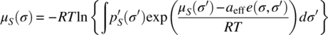
In this equation, μS(σ) is the chemical potential of an average molecular contact segment of size aeff in the ensemble S at temperature T, and e(σ,σ′) is the interaction energy functional e(σ,σ′) = emisfit(σ,σ′) + ehb(σ,σ′).
Since μS(σ) appears on both sides of Eq. (20.5), it must be solved by iteration, starting with μS(σ′) = 0 on the right‐hand side. Fortunately, the solution converges rapidly, and μS(σ) can be computed up to numerical precision within milliseconds on a personal computer. For a formal derivation of Eq. (20.5), we refer to Ref. [4].
Now it is straightforward to define the chemical potential of a solute X in the ensemble S by
where the residual part, i.e. the part resulting from the interactions of the surfaces in the liquid, is given by the surface integral of function μS(σ) over the solute surface, which is expressed using the σ‐profile of the solute in Eq. (20.6). The second part is the combinatorial contribution, which arises from the different shapes and sizes of the solute and solvent molecules. Expressions based on the surface areas and volume ratios of solvents and solutes, similar to standard chemical engineering expressions as Staverman–Guggenheim, are used in the context of COSMO‐RS [6]. COSMO surface areas and volumes are used for the evaluation of the combinatorial term. Hence Eq. (20.6) can be completely evaluated based on the information resulting from the COSMO calculations of the individual compounds.
The chemical potential of Eq. (20.6) is a pseudo‐chemical potential [7], i.e. the standard chemical potential without the concentration term RT ln xi. We will shortly use the term chemical potential for the pseudo‐chemical potential from Eq. (20.6) throughout this contribution. Providing the chemical potential of an arbitrary compound X in almost arbitrary solvents and mixtures as a function of temperature and concentration, Eq. (20.6) allows for the prediction of almost all thermodynamic properties of compounds or mixtures, such as activity coefficients, partition coefficients, or solubility, as shown in the flowchart for a COSMO‐RS property prediction in Figure 20.3.

FIGURE 20.3 Flowchart of a property prediction procedure with COSMO and COSMO‐RS.
As mentioned above, the COSMO‐RS method depends on a small number of adjustable parameters. Some of the parameters are predetermined from physics, while others are determined from selected properties of mixtures. The parameters are not specific to functional groups or types of molecule. As a result, COSMO‐RS is the least parameterized of all quantitative methods for the prediction of chemical properties in the liquid phase [5].
20.1.4 Treatment of Conformers in COSMO‐RS
Many molecules can adopt more than one conformation, and different conformers of one molecule can have different σ‐profiles. The chemical potentials of the individual conformers and hence the conformer distribution as well as the chemical potential of the compound represented by an ensemble of conformers depend on the composition of the system and the temperature. Thus, it is essential for property prediction with COSMO‐RS to take conformers with different σ‐profiles into account, each described by individual quantum chemical COSMO calculations. The relative contributions of the conformers are determined by an iterative procedure using the Boltzmann weight of the free energies of the conformers in the liquid phase. This results in a thermodynamically fully consistent treatment of multiple molecular conformations.
20.2 SOLUBILITY PREDICTION WITH COSMO‐RS
For the calculation of the solubility ![]() of a liquid compound X in a solvent S, we require the chemical potentials of X in S and in its pure liquid state,
of a liquid compound X in a solvent S, we require the chemical potentials of X in S and in its pure liquid state, ![]() and
and ![]() . If
. If ![]() is sufficiently small, so that the solvent behavior of the X‐saturated solvent S is not significantly influenced by the solute X, then the decadic logarithm of the solubility is given by
is sufficiently small, so that the solvent behavior of the X‐saturated solvent S is not significantly influenced by the solute X, then the decadic logarithm of the solubility is given by
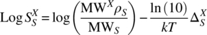
with the molecular weight MW, the solvent density ρ, and ![]() . In the case of high solubility (typically for solubility >10 wt. %), Eq. (20.7) becomes approximate, and the true solubility would have to be derived from a detailed search for a thermodynamic equilibrium of a solvent‐rich and a solute‐rich phase. But, in general, at least for the purpose of estimating drug solubility, Eq. (20.7) is sufficiently accurate.
. In the case of high solubility (typically for solubility >10 wt. %), Eq. (20.7) becomes approximate, and the true solubility would have to be derived from a detailed search for a thermodynamic equilibrium of a solvent‐rich and a solute‐rich phase. But, in general, at least for the purpose of estimating drug solubility, Eq. (20.7) is sufficiently accurate.
If the zeroth‐order ![]() as initially provided by Eq. (20.7), using infinite dilution of X in S, is resubstituted into the solubility calculation via
as initially provided by Eq. (20.7), using infinite dilution of X in S, is resubstituted into the solubility calculation via ![]() , a better approximation for
, a better approximation for ![]() is achieved. In other words, the solute chemical potential
is achieved. In other words, the solute chemical potential ![]() is computed for the solvent–solute mixture with the finite mole fraction of X in S that was predicted by the zeroth‐order
is computed for the solvent–solute mixture with the finite mole fraction of X in S that was predicted by the zeroth‐order ![]() . Then, using Eq. (20.7) with the new
. Then, using Eq. (20.7) with the new ![]() and the resulting values, an improved solubility
and the resulting values, an improved solubility ![]() is computed. Iterating this process to convergence, an iterative solubility can be achieved, which is also implemented in our COSMO‐RS program COSMOtherm and allows for the accurate prediction of solubility values even for cases of high solubility (solubility up to 50 wt. %). Thus, except for rare cases of very high solubility, a complicated search for a multiphase thermodynamic equilibrium of a solvent‐rich and a solute‐rich phase can be avoided, but instead Eq. (20.7) and its iterative refinement can be used.
is computed. Iterating this process to convergence, an iterative solubility can be achieved, which is also implemented in our COSMO‐RS program COSMOtherm and allows for the accurate prediction of solubility values even for cases of high solubility (solubility up to 50 wt. %). Thus, except for rare cases of very high solubility, a complicated search for a multiphase thermodynamic equilibrium of a solvent‐rich and a solute‐rich phase can be avoided, but instead Eq. (20.7) and its iterative refinement can be used.
Drugs are mostly solid at room temperature. Because the solid state of a compound X is related to its liquid state by the free energy difference ![]() , which is positive in the case of solids, a more general expression for solubility reads
, which is positive in the case of solids, a more general expression for solubility reads
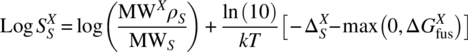
For liquid compounds, ![]() is negative and Eq. (20.8) reduces to Eq. (20.7).
is negative and Eq. (20.8) reduces to Eq. (20.7).
If melting point temperature Tmelt and heat of fusion ΔHfus or entropy of fusion ΔSfus are known experimentally for a solid compound, the free energy of fusion ΔGfus in Eq. (20.8) can be estimated from

or
Equations (20.9) and (20.10) can be complemented by an additional temperature‐dependent term using the heat capacity of fusion ΔCpfus in order to obtain good absolute predictions, but data for ΔCpfus are rarely available from experiment.
The free energy of fusion of new compounds is often not known, because experimental measurements can be cumbersome and substance may be scarce. Computational prediction of ![]() requires evaluation of the free energy of a molecule of compound X in its crystal, i.e. the crystal structure needs to be known or predicted. In general however, crystal structure prediction in particular for larger drugs is not yet feasible from a practical viewpoint due to the involved complexity. As an alternative, a QSPR approximation for ΔGfus can be used in COSMOtherm, which is based on a few rather obvious factors that should influence crystallization. Larger molecules should have larger ΔGfus than smaller ones, compounds with more polarity and hydrogen bonding ability should have larger ΔGfus than less polar ones, and also rigidity should give rise to larger ΔGfus. We found that a good regression equation for
requires evaluation of the free energy of a molecule of compound X in its crystal, i.e. the crystal structure needs to be known or predicted. In general however, crystal structure prediction in particular for larger drugs is not yet feasible from a practical viewpoint due to the involved complexity. As an alternative, a QSPR approximation for ΔGfus can be used in COSMOtherm, which is based on a few rather obvious factors that should influence crystallization. Larger molecules should have larger ΔGfus than smaller ones, compounds with more polarity and hydrogen bonding ability should have larger ΔGfus than less polar ones, and also rigidity should give rise to larger ΔGfus. We found that a good regression equation for ![]() can be achieved by a combination of the descriptors VX (the cavity volume from the COSMO calculation as size descriptor),
can be achieved by a combination of the descriptors VX (the cavity volume from the COSMO calculation as size descriptor), ![]() (the number of ring atoms in X as a descriptor of the compounds’ rigidity), and
(the number of ring atoms in X as a descriptor of the compounds’ rigidity), and ![]() (the compounds’ chemical potential in water as a combined measure of polarity and hydrogen bonding) [8]:
(the compounds’ chemical potential in water as a combined measure of polarity and hydrogen bonding) [8]:
20.2.1 Relative Solubility and Solubility Screening
The computational prediction of the relative solubility of a drug candidate in a variety of solvents with COSMO‐RS is straightforward and can be done without wasting any of the substance in this step. The required DFT/COSMO calculations can be done even before the compound comes to the development laboratory, and a COSMO‐RS solubility screening can be already completed when the work in the development department starts.
Experimental data for melting point and free energy of fusion can often be obtained through differential scanning calorimetry. If melting point temperature and heat of fusion or entropy of fusion are known for the compound in question, the free energy of fusion ΔGfus can be calculated according to Eq. (20.9) or (20.10), and a solubility screening for absolute solubilities can be done. If data for ΔGfus are not known, an estimated ΔGfus may be used, either from the QSPR model implemented in COSMOtherm or from an external model.
FIGURE 20.4 Database view in COSMOthermX. Databases can be searched and columns are sortable.
FIGURE 20.5 Overview of COSMOthermX with compound list, solubility panel, and input section. When the solute state is set to liquid, ΔGfus = 0 is used, while with solid solute state, given or estimated values for ΔGfus are used. The iterative refinement can also be set in the solubility panel. In the solvent frame, the solvent composition is set to pure for the respective solvent. Pictured here are settings for absolute solubility using the iterative refinement procedure.
FIGURE 20.6 Excerpt from the COSMOtherm table file for the solubility calculation of acetaminophen in pure solvents. Log10(x_solub) indicates the logarithmic solubility in mole fractions.
TABLE 20.1 Experimental, Predicted Relative, and Predicted Absolute Solubilities of Acetaminophen in Pure Solvents
Source: Data from Granberg and Rasmuson [9].
| Solvent | Experimental | Predicted Relative | Predicted Absolute | Error | |||||
| cS (g/kg) | Log S(mg/g) | Log S(x) | S (mg/g) | Log S (mg/g) | Log S(x) | S (mg/g) | Log S (mg/g) | ||
| Water | 17.39 | 1.24 | −1.6819 | 174.53 | 2.24 | −3.0745 | 7.07 | 0.85 | −0.39 |
| Methanol | 371.61 | 2.57 | 0.6155 | 19 465.33 | 4.29 | −1.0119 | 459.02 | 2.66 | 0.09 |
| Ethanol | 232.75 | 2.37 | 0.4809 | 9929.62 | 4.00 | −1.0687 | 280.11 | 2.45 | 0.08 |
| 1,2‐Ethanediol | 144.3 | 2.16 | 0.1829 | 3711.29 | 3.57 | −1.2535 | 135.86 | 2.13 | −0.03 |
| 1‐Propanol | 132.77 | 2.12 | 0.2182 | 4157.36 | 3.62 | −1.2441 | 143.37 | 2.16 | 0.03 |
| 2‐Propanol | 135.01 | 2.13 | 0.3858 | 6115.50 | 3.79 | −1.1268 | 187.86 | 2.27 | 0.14 |
| 1‐Butanol | 93.64 | 1.97 | 0.0690 | 2390.35 | 3.38 | −1.3675 | 87.50 | 1.94 | −0.03 |
| 1‐Pentanol | 67.82 | 1.83 | −0.0639 | 1480.10 | 3.17 | −1.4866 | 55.92 | 1.75 | −0.08 |
| 1‐Hexanol | 49.71 | 1.70 | −0.1756 | 987.32 | 2.99 | −1.5932 | 37.75 | 1.58 | −0.12 |
| 1‐Heptanol | 37.43 | 1.57 | −0.2630 | 709.92 | 2.85 | −1.6779 | 27.31 | 1.44 | −0.14 |
| 1‐Octanol | 27.47 | 1.44 | −0.3589 | 507.95 | 2.71 | −1.7716 | 19.64 | 1.29 | −0.15 |
| Acetone | 111.65 | 2.05 | 0.9328 | 22 297.15 | 4.35 | −0.8016 | 411.01 | 2.61 | 0.57 |
| 2‐Butanone | 69.99 | 1.85 | 0.6508 | 9380.65 | 3.97 | −0.9153 | 254.79 | 2.41 | 0.56 |
| 4‐Methyl‐2‐pentanone | 17.81 | 1.25 | 0.1126 | 1956.04 | 3.29 | −1.2844 | 78.41 | 1.89 | 0.64 |
| Tetrahydrofuran | 155.37 | 2.19 | 1.6842 | 101 306.53 | 5.01 | 0.0527 | 2366.72 | 3.37 | 1.18 |
| 1,4‐Dioxane | 17.08 | 1.23 | 1.0644 | 19 898.20 | 4.30 | −0.7332 | 317.14 | 2.50 | 1.27 |
| Ethyl acetate | 10.73 | 1.03 | 0.0872 | 2097.21 | 3.32 | −1.2415 | 98.38 | 1.99 | 0.96 |
| Acetonitrile | 32.83 | 1.52 | 0.1079 | 4720.92 | 3.67 | −1.2689 | 198.25 | 2.30 | 0.78 |
| Diethylamine | 1316.9 | 3.12 | 3.5201 | 6 845 852.30 | 6.84 | 1.4457 | 57 683.45 | 4.76 | 1.64 |
| N,N‐Dimethylformamide | 1012.02 | 3.01 | 2.2018 | 276 105.51 | 5.44 | 0.4567 | 4965.64 | 3.70 | 0.69 |
| Dimethyl sulfoxide | 1132.56 | 3.05 | 3.3062 | 3 915 389.90 | 6.59 | 0.2699 | 3601.53 | 3.56 | 0.50 |
| Acetic acid | 82.72 | 1.92 | 0.3232 | 5298.62 | 3.72 | −1.1632 | 172.87 | 2.24 | 0.32 |
| Dichloromethane | 0.32 | −0.49 | −1.8354 | 26.00 | 1.41 | −3.1820 | 1.17 | 0.07 | 0.56 |
| Chloroform | 1.54 | 0.19 | −1.8884 | 16.37 | 1.21 | −3.2647 | 0.69 | −0.16 | −0.35 |
| Carbon tetrachloride | 0.89 | −0.05 | −4.5149 | 0.03 | −1.52 | −5.9289 | 0.00 | −2.94 | −2.89 |
| Toluene | 0.34 | −0.47 | −3.0598 | 1.43 | 0.16 | −4.4573 | 0.06 | −1.24 | −0.77 |
Log S(x) indicates the logarithmic solubility in mole fractions.
FIGURE 20.7 Predicted relative solubility of acetaminophen versus experimental data in pure solvents at 303.15 K. Triangles represent relative solubility data, with empty triangles (Δ) representing alcoholic solvents and water and solid triangles (▴) representing the remainder of the solvent data set. One outlier (carbon tetrachloride) is represented by a solid diamond (♦).
FIGURE 20.8 Predicted absolute solubility of acetaminophen versus experimental data in pure solvents at 303.15 K. Empty triangles (Δ) represent absolute solubility data of alcoholic solvents and water; solid triangles (▴) represent the remainder of the solvent data set. Four outliers (carbon tetrachloride, diethylamine, 1,4‐dioxane, tetrahydrofuran) represented by solid diamonds (♦).

FIGURE 20.9 Input section of COSMOthermX with entries for a list of solvent compositions.
FIGURE 20.10 Excerpt from the COSMOtherm table file for the solubility calculation of acetaminophen in a binary solvent system.
TABLE 20.2 Experimental and Predicted Solubilities of Acetaminophen in Water–Acetone and Acetone–Toluene Binary Solvent Mixtures
Source: Data from Granberg and Rasmuson [14].
| % Mass Fraction | Experimental | Predicted | Error | |||||
| Water | Acetone | Toluene | cS (g/kg) | Log S (mg/g) | Log S(x) | S (mg/g) | Log S (mg/g) | |
| 100 | 0 | 0 | 14.90 | 1.17 | −3.1508 | 5.93 | 0.77 | −0.40 |
| 93 | 7 | 0 | 28.18 | 1.45 | −2.7658 | 13.69 | 1.14 | −0.31 |
| 85 | 15 | 0 | 53.0 | 1.72 | −2.3994 | 29.99 | 1.48 | −0.25 |
| 80 | 20 | 0 | −2.1978 | 45.87 | 1.66 | 1.66 | ||
| 75 | 25 | 0 | −2.0125 | 67.47 | 1.83 | 1.83 | ||
| 70 | 30 | 0 | 150.0 | 2.18 | −1.8424 | 95.66 | 1.98 | −0.20 |
| 65 | 35 | 0 | −1.6879 | 130.58 | 2.12 | 2.12 | ||
| 60 | 40 | 0 | −1.5500 | 171.24 | 2.23 | 2.23 | ||
| 55 | 45 | 0 | −1.4290 | 215.47 | 2.33 | 2.33 | ||
| 50 | 50 | 0 | 327.0 | 2.51 | −1.3242 | 260.58 | 2.42 | −0.10 |
| 30 | 70 | 0 | 454.6 | 2.66 | −1.0260 | 408.68 | 2.61 | −0.05 |
| 15 | 85 | 0 | 420.3 | 2.62 | −0.8851 | 452.18 | 2.66 | 0.03 |
| 7 | 93 | 0 | 302.2 | 2.48 | −0.8364 | 438.41 | 2.64 | 0.16 |
| 3 | 97 | 0 | 197.1 | 2.29 | −0.8247 | 415.72 | 2.62 | 0.32 |
| 0 | 100 | 0 | 99.8 | 2.00 | −0.8285 | 386.32 | 2.59 | 0.59 |
| 0 | 95 | 5 | 91.7 | 1.96 | −0.8517 | 359.46 | 2.56 | 0.59 |
| 0 | 90 | 10 | 82.4 | 1.92 | −0.8774 | 332.39 | 2.52 | 0.61 |
| 0 | 85 | 15 | 75.7 | 1.88 | −0.9062 | 305.14 | 2.48 | 0.61 |
| 0 | 80 | 20 | 66.4 | 1.82 | −0.9386 | 277.63 | 2.44 | 0.62 |
| 0 | 70 | 30 | 52.8 | 1.72 | −1.0165 | 222.79 | 2.35 | 0.63 |
| 0 | 60 | 40 | 37.08 | 1.57 | −1.1186 | 168.79 | 2.23 | 0.66 |
| 0 | 50 | 50 | 26.56 | 1.42 | −1.2563 | 117.58 | 2.07 | 0.65 |
| 0 | 30 | 70 | 8.55 | 0.93 | −1.7149 | 37.19 | 1.57 | 0.64 |
| 0 | 20 | 80 | 3.39 | 0.53 | −2.1018 | 14.50 | 1.16 | 0.63 |
| 0 | 15 | 85 | 2.12 | 0.33 | −2.3663 | 7.68 | 0.89 | 0.56 |
| 0 | 7 | 93 | 0.78 | −0.11 | −2.9938 | 1.73 | 0.24 | 0.35 |
| 0 | 0 | 100 | 0.37 | −0.43 | −4.6734 | 0.03 | −1.46 | −1.03 |
Log S(x) indicates the logarithmic solubility in mole fractions.
FIGURE 20.11 Experimental and predicted solubility of acetaminophen in acetone–water binary mixtures at 298.15 K. Diamonds (◊) are experimental data; the solid line is from the model prediction.
FIGURE 20.12 Experimental and predicted solubility of acetaminophen in toluene–acetone binary mixtures at 298.15 K. Diamonds (◊) are experimental data; the solid line is from the model prediction.
20.3 CHEMICAL REACTIONS IN SOLUTION
Calculation of reaction energies in the gas phase is a standard application in quantum chemistry. The computational prediction of free energies of reaction in solution is more involved, but still a rather straightforward procedure. Generally, the free energy of reaction is the difference of the total free energies of the reactants and the products of the reaction. For a reaction
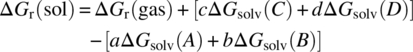
where A and B are the reactants with stoichiometric coefficients a and b and C and D are the reaction products with stoichiometric coefficients c and d, the free energy of reaction can be calculated from the difference of the sums of free energies on both sides of the reaction:
The free energies of the reactants and products, and thus the free energy of reaction, depend on the conditions under which the reaction takes place. The free energy of reaction in the gas phase differs from the free energy of reaction in solution, and it is different in each specific solvent.
In solution, the Gibbs free energy of a species is
Here Egas(i) is the gas‐phase energy of the compound, and for computational predictions of the reaction free energy, it should be taken from an adequate quantum chemical (DFT or post‐Hartree–Fock) level. ΔGsolv(i), the free energy of solvation, describes the change of the free energy that occurs when the compound is dissolved from the gas phase into the liquid phase. This contribution to the total free energy of a compound can be computed using COSMO‐RS.
Using the gas‐phase energies of the compounds and the free energies of solvation of the compounds, the free energy of reaction in solution can be calculated according to a thermodynamic cycle as depicted in Figure 20.13.
FIGURE 20.13 Cycle for computation of a free energy change in solution.
In order to compute the lower horizontal leg of the cycle, corresponding to the reaction in solution, we have to take the appropriate sums and differences of the upper horizontal leg, i.e. the gas‐phase reaction, and the vertical legs, i.e. the solvation energies of the compounds:
ΔGr(gas) can be calculated from the chemical potential of the compounds in the gas phase. As already mentioned, the quantum chemical gas‐phase energy Egas of a compound is computed in vacuum at absolute zero. Furthermore, Egas does not account for vibrational motion that is present even at T = 0 K. The so‐called zero‐point energy or zero‐point vibrational energy (ZPE) can be computed quantum chemically from the vibrational frequencies of the compound and is a standard correction to Egas. Using the ZPE, the free energy of a compound can be calculated as
As a further refinement for the gas‐phase energies of the compounds and the resulting reaction energy, the temperature‐dependent thermal contributions to the free energy μvib of the molecule can be calculated. From vibrational frequencies, the molecular translational, rotational, and vibrational partition functions, qtrans, qrot, and qvib, can be calculated, thus enabling prediction of thermodynamic functions at temperatures other than 0 K and finite pressure:

The other terms required for Eq. (20.15), the free energies of solvation ΔGsolv, can be obtained from a COSMOtherm prediction of the reverse process, i.e. from a vapor pressure prediction. The partial vapor pressure P(i) that is calculated by COSMOtherm corresponds to the pure compound vapor pressure times the activity coefficient and is related to ΔGsolv by
with P being the reference pressure at which the reaction takes place.
Note that if the reactant or product compounds are present in the mixture at a finite concentration with a mole fraction x(i) (e.g. if the reaction takes place in bulk reactant liquid), an entropic contribution RT ln(x(i)) of the compound has to be added to the compounds’ free energy G(i).
20.3.1 Heat of Reaction
The heat of reaction or reaction enthalpy in solution can be calculated by a procedure similar to the free energy of reaction. Instead of the free energy of solvation of the compounds, we make use of the heat of vaporization ΔHvap. Since ΔHvap is the enthalpy that is needed to transfer the compound from the liquid phase to the gas phase, it has to be subtracted from the gas‐phase energy to obtain the enthalpy of the compound in solution:
ZPE corrections or thermal correction terms for the enthalpy in the gas phase can also be used as corrections to the gas‐phase energies of the compounds for the calculation of the heat of reaction.
Similarly to Eq. (20.13) for the free energy of reaction ΔGr, the heat of reaction ΔHr can be calculated from the enthalpy of the compounds:
20.3.2 Equilibrium Constants
The equilibrium constant K of a reaction is related to the free energy of reaction by
For a reaction in an ideal solution, i.e. in infinite dilution, the equilibrium constant can be calculated using the reaction free energy in solution according to Eq. (20.15). The free energies of the individual compounds can be computed using different quantum chemical correction terms as described above.
20.3.3 Accuracy
In the described procedure the free energies of the compounds are calculated from two main contributions, the quantum chemical gas‐phase energy and the free energy of solvation. The accuracy of the resulting reaction energy is determined mainly by the accuracy of the underlying quantum chemical method. With DFT methods like the BP86 functional, errors of the absolute reaction energy can be in the range of 10 kcal/mol or more [15, 16]. However, for relative reaction energies of one reaction in different solvents in a solvent screening application, i.e. if we are looking at the variation of the solvation energy only, calculated as the COSMOtherm contribution in the liquid phase, the accuracy is much higher. For such relative reaction energy predictions considering ΔGsolv or ΔHvap from the COSMOtherm vapor pressure prediction only, an accuracy of 0.5 kcal/mol can be expected.
For a higher accuracy of absolute predictions of the reaction energy or enthalpy, it follows that a more accurate quantum chemical method should be applied for the calculation of the gas‐phase energy, e.g. the MP2 or coupled‐cluster methods combined with adequate basis sets. Quantitative improvement of the total free energy of a compound G(i) can also be achieved by the ZPE and thermal corrections to the gas‐phase energy of the compound.
20.3.4 Calculation of the Free Energy of Reaction and Heat of Reaction
A procedure for the computational prediction of the free energy of reaction ΔGr or heat of reaction ΔHr using quantum chemical gas‐phase energies and free energies of solvation or heats of vaporization from COSMO‐RS is described in the following:
- Compute the reactant and product molecules using the DFT methods for which COSMOtherm is parameterized. Both COSMO and gas‐phase quantum chemical calculations are required. Then use COSMOtherm to obtain the ΔGsolv and/or ΔHvap values.
- Compute gas‐phase energies Egas of the reactant and product molecules with a high‐level ab initio method, e.g. the coupled‐cluster method.
- Compute vibrational frequencies for reactant and product molecules to obtain the ZPE correction or the thermal corrections to the gas‐phase energies of the compounds. Vibrational frequency calculations at a DFT level of theory are usually sufficiently accurate.
- Combine Egas, ZPE or thermal corrections, and ΔGsolv to compute the compounds G(i) according to Eqs. (20.16) and (20.17) or Egas, ZPE or thermal corrections, and ΔHvap to compute the compounds H(i).
- Calculate the free energy of reaction ΔGr or the heat of reaction ΔHr from the difference of the sums of free energies or enthalpies on both sides of the reaction as described by Eqs. (20.13) and (20.20).

FIGURE 20.14 Excerpt from the mixture output section of the COSMOtherm output file for a vapor pressure calculation of compounds in pure tetrahydrofuran at 25 °C.
TABLE 20.3 Gas‐Phase Energies, Heat of Vaporization, Zero‐Point Vibrational Energies, Thermal Corrections, Total Enthalpies of Compounds, and Heat of Reaction for the Hydrogenation of Nitrobenzene
| 1 | 2 | 3 | 4 | ΔHr | ||
| MP2/TZVPP | (BP86/TZVP) | |||||
| Hvap | 12.02 | 1.35 | 14.54 | 10.24 | ||
| Egas (BP86/TZVP) (Hartree) | −436.944 122 | −1.177 446 | −287.715 215 | −76.465 165 | ||
| Egas (MP2/TZVPP) (Hartree) | −435.958 485 | −1.164 647 | −287.000 283 | −76.323 461 | ||
| ZPE (BP86/TZVP) (Hartree) | 0.099 295 | 0.009 850 | 0.113 236 | 0.020 640 | ||
| ΔHT (thermal corrections) | 67.36 | 8.26 | 75.45 | 15.32 | ||
| H = Egas − Hvap | −273 580.11 | −732.17 | −180 109.95 | −47 903.93 | −141.19 | (−125.06) |
| H = Egas + ZPE − Hvap | −273 517.80 | −725.99 | −180 038.89 | −47 890.98 | −125.08 | (−108.95) |
| H = Egas + ΔHT − Hvap | −273 512.75 | −723.92 | −180 034.50 | −47 888.61 | −127.22 | (−111.09) |
Enthalpy terms are in kcal/mol; quantum chemical gas‐phase energies and ZPE are in Hartree.
FIGURE 20.15 Catalytic transamination of 1‐methoxy‐2‐propanone and isopropylamine.
FIGURE 20.16 Excerpt from the mixture output section of the COSMOtherm output file for a vapor pressure calculation of compounds in pure water at 50 °C.
TABLE 20.4 Energy Terms and Energy Corrections for the Reactants and Products for Reaction 2 and Free Energies of Reaction with the Various Correction Terms
| 1 | 2 | 3 | 4 | ΔGr | ln K | |
| Log10(P(i) [mbar]) | 2.720 32 | 4.112 02 | 3.123 39 | 3.755 18 | ||
| Gsolv | −0.41 | 1.64 | 0.18 | 1.12 | ||
| Egas (MP2/TZVPP) (Hartree) | −307.100 753 | −174.113 883 | −288.440 644 | −192.779 317 | ||
| ZPE (BP86/TZVP) (Hartree) | 0.112 968 | 0.117 222 | 0.149 297 | 0.080 872 | ||
| μvib (thermal corrections) | 54.44 | 227.770 | 71.54 | 32.03 | ||
| G = Egas (MP2) + Gsolv | −192 709.05 | −109 256.47 | −180 999.06 | −120 969.74 | −3.27 | 5.10 |
| G = Egas (MP2) + Gsolv + ZPE | −192 638.16 | −109 182.91 | −180 905.38 | −120 918.99 | −3.29 | 5.12 |
| G = Egas (MP2) + Gsolv + μvib | −192 660.99 | −109 202.03 | −180 927.52 | −120 937.70 | −2.20 | 3.43 |
| Relative amount of compound in equilibrium | 0.08 | 0.08 | 0.42 | 0.42 |
The relative amount of the compounds in equilibrium has been calculated from the equilibrium constant ln K = 3.43. Free energy terms and chemical potential are in kcal/mol; quantum chemical gas‐phase energies and ZPE are in Hartree.
20.4 SCREENING OF CO‐CRYSTALS
Co‐crystalline materials consisting of an active pharmaceutical ingredient (API) and an excipient, usually termed coformer (co‐crystal former), have attracted strong interest in recent years by pharmaceutical research and development. This is mostly due to the fact that co‐crystals provide a leverage to modify the physicochemical properties of a drug substance, in particular its solubility and dissolution behavior and hence its bioavailability. In addition, they open up new interesting possibilities from an intellectual property and patent perspective. This has generated the need for the rational design of such systems and for approaches that go beyond a simple trial‐and‐error process.
The application of COSMO‐RS theory to this field emerged rather recently when it was demonstrated that the excess enthalpy (or mixing enthalpy) of the supercooled co‐crystal melt as computed by COSMOtherm gives rather good correlation with the materials’ tendency to co‐crystallize [19].
The excess enthalpy Hex of a mixture is defined as the enthalpy difference between the mixture (Hmix) and the pure state (Hpure) for each component i with mole fraction xi:
The excess enthalpy Hex corresponds to the mixing enthalpy ΔHmix of the system, whereas the latter usually refers to integer moles of the reactants. The more negative the excess enthalpy, the more the compounds prefer the mixture over their pure states. In this respect Hex of a binary system may also be understood as a quantifier of complementarity of two structures. Figure 20.17 shows a histogram of the computed Hex for about 500 molecule pairs including experimentally confirmed co‐crystals (blue) and failed co‐crystallization attempts (red). It is quite apparent that there is a significant correlation with the tendency to co‐crystallize, in particular at regions with strongly negative Hex. For positive Hex co‐crystal formation becomes significantly less probable, whereas in the area slightly below 0 kcal/mol, the discrimination between co‐crystals and non‐co‐crystals is more difficult. A similar picture as in 4.1 would be obtained using the Gibbs free energy of mixing ΔGmix, which is related to Hex:

FIGURE 20.17 Histogram and normalized probability distribution for the computed excess enthalpy of a set of about 500 co‐crystal experiments.
Here, Gex is the excess free energy and Sex the excess entropy in the mixture. In retrospective, the relation of liquid‐phase properties with co‐crystal formation can be better understood by the examination of the thermodynamic cycle for co‐crystallization (Figure 20.18) that links the free energy of co‐crystal formation ΔrGcocrystal to the free energy of mixing ΔGmix.

FIGURE 20.18 Thermodynamic cycle for the formation of co‐crystals AmBn out of components A and B via a hypothetical supercooled liquid state. The free energy of fusion ΔGfus is the energy that is needed to convert the material from the solid state into the supercooled liquid state (sc. liquid) at a specific temperature T.
In this thought experiment the drug A and the coformer B are transferred into their respective supercooled liquid state by expending the free energy of fusion ΔGfus. Mixing of A and B yields the co‐crystal AmBn in its supercooled liquid state (ΔGmix), which then upon solidification gives the final co‐crystal. The correlation of the mixing or excess energies (Hex,ΔGmix) with co‐crystal formation can be explained by the assumption that the remaining terms, the sum of ΔGfus(A) and ΔGfus(B) of reactants A and B, and the −ΔGfus(AB) of the co‐crystal are of similar magnitude and hence cancel each other partially when going along the thermodynamic cycle:
Hence, the term ΔΔGfus (or at least its variance) needs to be small compared with ΔGmix in order to have a good prediction (ranking). Furthermore, the overall entropic changes related to the conversion of solids A and B to solid AmBn will be comparably small; thus the enthalpy, i.e. Hex, and not the free energy should be the prevailing quantity in this process. Although the drug–coformer interaction in co‐crystals is in many cases dominated by intermediate to strong hydrogen bonding, electrostatics and vdW interaction also play an important role in the condensed state, all of which are properly taken into account by COSMO‐RS theory.
So far only thermodynamic effects have been considered; kinetic effects however may also play a role for crystallization. Therefore, for rather large molecules, it is recommended to introduce an additional term, i.e. a penalty, that takes into account the molecular flexibility that poses a major barrier for crystallization. It was found that using this number of rotatable bonds as a simple additional linear term gives an improvement in predictivity for flexible systems. This can be rationalized by the assumption that the probability of crystallization is an exponentially decreasing function of the molecular flexibility that becomes an essentially linear term when being converted to the energy domain.
Table 20.5 shows the result of the excess enthalpy‐based screening for the anti‐malaria drug artemisinin against 67 potential coformers. Experimentally only two co‐crystals, namely, resorcinol and orcinol, have been found. The data from the experimental screening has been taken from the study of Karki et al. [20].
TABLE 20.5 Results of the Co‐crystal Screening for the Anti‐malaria Drug Artemisinin and 67 Coformers, Where for the Sake of Conciseness Only the Top and the Bottom of the Whole Coformer Set Are Presented
Source: Experimental data taken from Ref. [19].
| Rank | Coformer | Co‐crystal | Hex (kcal/mol) |
| 1 | Ethanedisulfonic acid | No | −3.86 |
| 2 | 1,3‐Dihydroxynaphthalene | No | −2.93 |
| 3 | Phloroglucinol | No | −2.53 |
| 4 | Benzenesulfonic acid | No | −2.01 |
| 5 | Resorcinol | Yes | −1.98 |
| 6 | Olivetol | No | −1.94 |
| 7 | Orcinol | Yes | −1.84 |
| 8 | Gentisic acid | No | −1.80 |
| 9 | Cyanuric acid | No | −1.78 |
| 10–63 | … | No | … |
| 64 | Lysine | No | 0.78 |
| 65 | Arginine | No | 0.82 |
| 66 | L‐Serine | No | 0.82 |
| 67 | Alanine | No | 0.92 |
Coformers are sorted due to increasing excess enthalpy.
Both experimentally confirmed co‐crystals are placed at the fifth and seventh positions on the whole list of 67 tested coformers. This highlights the basic idea of a COSMO‐RS‐based prescreening that is not to obtain absolute predictions but to improve the chances to successfully find a coformer for a follow‐up experimental search. As expected it shows some disagreement with experiment, which has mainly two reasons. Firstly, several approximations have been made from a model point of view, the severest one certainly the total neglect of crystalline long‐range order. Secondly, from an experimental point of view, it can never be ruled out that some of the low excess enthalpy pairs indeed form a co‐crystal that just has not been found in the experiment. Hence, it is possible that some of the false‐positive low excess pairs may still form a co‐crystal at the right experimental conditions. In this context a study by Corner et al. has to be mentioned where COSMOtherm was used to prescreen coformers for the highly polymorphic drug precursor ROY [21]. Here, one of the top predicted coformers (pyrogallol) did not form a co‐crystal but instead an amorphous complex with ROY. In other words, ROY could be stabilized in its amorphous form due to a COSMOtherm‐predicted strong intermolecular interaction with pyrogallol. This is an important finding considering that usually the amorphous form shows a higher solubility/bioavailability than its crystalline counterparts.
So far, the excess enthalpy is merely a quantity that ranks the potential coformers relatively and does not give absolute prediction or 1/0 classification of co‐crystal formation. However, according to Figure 20.17, the probability to form a co‐crystal decreases strongly close above 0 kcal/mol, and pairs having a positive excess enthalpy can be ruled out as co‐crystal formers with high confidence. The introduction of a fixed optimal threshold for a co‐crystal vs. non‐co‐crystal classification is possible, but the exact size of the threshold may vary with the specific targeted drug under consideration.
A thorough statistical analysis of a whole array of drug and coformer sets has been carried out in Reference [19] and in [23] using the area under the curve (AUC) metric from a receiver operating characteristic (ROC) curve. Using an up‐to‐date COSMOtherm parameterization, the overall performance including the penalty term amounts to an AUC of about 0.83 (AUC = 0.81 without the penalty term) on a set of 20 drugs. In other words, the approach ranks any drug–excipient pair that forms a co‐crystal before any non‐co‐crystal pair by a probability of about 83%.
An interesting aspect is related to the original objective of improving solubility via transferring the drug into a co‐crystal: apart from kinetic effects during dissolution, the thermodynamic solubility can only be improved as compared with the pure drug if there is significant interaction between drug and coformer in solution, thereby reducing the activity of the drug as compared with its state without the coformer. This will however strongly correlate with the strength of the excess enthalpy. Hence screening for low excess enthalpy mixtures will simultaneously improve the chance of finding coformers that improve the overall solubility.
Solvates are strongly related to co‐crystal as they differ only by the fact that one of the components is liquid at room temperature. Consequently, some attempts have been undertaken to correlate the excess enthalpy with the tendency of a drug to form a solvate [19, 24]. Again, the correlation is significant, however in many cases less pronounced than for co‐crystals. Usually interactions between solvents and drug are smaller than for coformer and drug, and packing effects are more important. In particular solvents having the right shape to fit into voids or channels of the crystalline may form inclusion compounds in the crystalline state that will show a Hex close to zero and hence are out of the scope of the current approach. However, it was shown recently that overall predictions can be improved by considering the shape of the solvents and the topology of the drug [25].
A special subset of solvates are hydrates where the solvent that crystallizes together with the drug is water. Abramov tested the excess enthalpy approach for a set of 61 diverse hydrate‐ and non‐hydrate‐forming drugs [22]. The aim of this study was to predict not only the propensity of the pharmaceutical compounds to form a hydrate but also the resistance of co‐crystals to hydration at high humidity conditions. Besides Gex and Hex, also other descriptors were taken into account such as the octanol–water partition coefficient (clog P), topological surface area (TPSA), and different donor–acceptor counts.
As a result it was demonstrated that the excess energy approach based on COSMO‐RS offers the most efficient way to probe the tendency of a drug to form a hydrate. Moreover, for the investigated caffeine and theophylline co‐crystals, the size of the excess enthalpy correlated well with the improved resistance toward hydration at 98% RH conditions.
TABLE 20.6 COSMO‐RS‐Based Co‐crystal Screening for Bicalutamide (Example Problem 20.5)
| Coformer | Hex (kcal/mol) | Co‐crystal |
| 1,2‐Bis(4‐pyridyl)ethane | −1.57 | 0 |
| trans‐1,2‐Bis(4‐dipyridyl)ethylene | −1.21 | 1 |
| 4,4′‐Bipyridine | −1.13 | 1 |
| 1‐Naphthol | −0.99 | 0 |
| 1,3,5‐Trihydroxybenzene | −0.89 | 0 |
| 4,4‐Biphenol | −0.71 | 0 |
| 4‐Phenylpyridine | −0.68 | 0 |
| 1,3‐Dihydroxybenzene | −0.62 | 0 |
| 4‐Cyanopyridine | −0.24 | 0 |
| 3‐Cyanopyridine | −0.19 | 0 |
| 3‐Cyanophenol | 0.01 | 0 |
| 1‐Naphtalenecarbonitrile | 0.01 | 0 |
| 4‐Cyanophenol | 0.10 | 0 |
| 1,3‐Benzenedicarbonitrile | 0.13 | 0 |
| 1,4‐Benzenedicarbonitrile | 0.13 | 0 |
| 3‐Hydroxypyridine | 0.30 | 0 |
| 5‐Hydroxyisoquinoline | 0.31 | 0 |
| 1‐Hexadecanol | 1.28 | 0 |
Entries are ordered by increasing excess enthalpy Hex.
20.5 CONCLUSION AND OUTLOOK
In this chapter we presented an overview of three different applications of COSMO‐RS in the drug development process. The power and main benefit of the COSMO‐RS model is that properties in solution can be obtained from ab initio calculation without any experimental input. It does not require external data for modeling and can also be used when empirical models are not parameterized. Complex multifunctional molecules and new chemical functionalities are treated on the same footing as simple organic molecules.
Prediction of relative drug solubility with COSMO‐RS is based on a consistent thermodynamic modeling of interactions in the solvent and the supercooled state of the drug. Solvent mixtures can be treated in the same way as pure solvents and with similar accuracy. Absolute solubility prediction is limited by the availability of free energy of fusion data.
Although COSMO‐RS in its present state cannot be proven to be more accurate than more empirical models with many adjusted parameters, its strength is the essential independency from experimental data. This allows for independent modeling and avoids errors resulting from erroneous experimental data on which empirical models rely. Potential improvement to the current COSMO‐RS solubility prediction model includes a more accurate fusion term for absolute solubility prediction, and improvement of the COSMO‐RS interaction terms themselves, and requires more reliable experimental data as are available at present.
With COSMO‐RS, solubility prediction is also possible for salts. This is important as many drugs are formulated as salts. Solvent systems involving ionic liquids can also be treated with very good accuracy [28]. Furthermore, different conformational forms of molecules can be used for solubility screening, and the relative weight of conformers in different solvents can be determined. This feature basically allows for examination of conditions influencing the crystallization process and solvent screening for conformational polymorphism and pseudopolymorphism.2
Another application of COSMO‐RS frequently used in pharmaceutical and agrochemical industry deals with reaction modeling. In principle, reaction equilibrium, mechanism, rate, and by‐product formation may be solvent dependent. Here we investigated the influence of solvation on the free energy and heat of reaction and the reaction equilibrium only. A straightforward procedure for the computational prediction of the free energy of reaction and heat of reaction has been shown, and the effect of the employed quantum chemical level on the absolute heat of reaction has been demonstrated. Elsewhere, it has been shown that although, depending on the quantum chemical level, absolute values for the free energy of reaction may differ substantially from experimental data, general trends are predicted correctly [29].
Finally, the prediction of co‐crystal formation can be carried out using COSMO‐RS. Although not being a mere solution process, it is however strongly related to it. In fact, the problem of co‐crystal formation that cannot be treated yet rigorously in all its complexity is approximated by assuming the co‐crystal to be a supercooled mixture of API and coformer. This is of course a strong simplification, with a larger error bar than the usual COSMO‐RS applications. Nevertheless, as it was demonstrated in this chapter, it allows to guide experimental work quite efficiently.
All applications of COSMO‐RS require quantum chemical calculations of compounds, taking into account the various molecular conformations of the compounds. This constitutes the computationally most demanding part of the procedure but has to be done only once per compound. The COSMO files of the involved compounds can be reused for other projects and all types of properties. Thus, if combined with a database of precalculated COSMO files for common compounds, thermodynamic property calculations with COSMOtherm can be carried out quite fast and efficiently.
20.A DETAILS OF COSMO AND GAS‐ PHASE CALCULATIONS
For later use of the COSMO files in COSMOtherm, the details of the quantum chemical COSMO calculation should be consistent with one of the parameterizations of COSMOtherm.
There are three levels of different qualities mainly used in COSMOtherm: a lower, computationally less expensive level; an intermediate level, which is sufficiently accurate for most problems; and a higher level, which is computationally more time consuming and also resolves some particular problem cases. As the intermediate level is a good compromise between accuracy and efficiency, it has been used throughout in this contribution and requires the following:
- BP86 DFT geometry optimization with a TZVP quality basis set and the RI approximation applied in the gas phase and in the conductor.
- For COSMO calculations only: COSMO applied in the conductor limit (ε = ∞) using optimized element‐specific COSMO radii for the cavity construction.
- If more than one conformation is considered to be potentially relevant for a compound, QC calculations have to be done for all conformations.
20.B STEPS FOR CALCULATING THE FREE ENERGY OR ENTHALPY OF A COMPOUND
Apart from the heat of vaporization or free energy of solvation that is calculated by COSMOtherm, the free energies and enthalpies of compounds involved in the reaction examples are composed from several quantum chemical contributions.
20.B.1 Gas‐Phase Energy
The BP86/TZVP gas‐phase energy is obtained from a gas‐phase geometry optimization of the compound using the settings described in Appendix 20.A. The resulting energy value can be found in output files of the TURBOMOLE program suite. The protocol file job.last comprises the output of the last complete cycle and information about the settings that were applied in the program run, e.g. convergence criteria. The gas‐phase energy can be read from “total energy” line in the output section displayed in Figure 20.B.1. If the graphical user interface TmoleX is used, the gas‐phase energy can also be taken from the Energy block of the Job Results panel. This panel also displays information about the run of the job (Figure 20.B.2).
FIGURE 20.B.1 Excerpt from the TURBOMOLE output file job.last from a BP86 gas‐phase geometry optimization of nitrobenzene.

FIGURE 20.B.2 Job Results panel of the graphical user interface TmoleX of the TURBOMOLE program suite.
The MP2/TZVPP gas‐phase energy is obtained from an MP2 geometry optimization employing the TZVPP basis set (also called def‐TZVPP) and the RI approximation. The module used for this type of calculation is ricc2 (Figure 20.B.3). In TmoleX, the method has to be set to RI‐MP2 in the “Level” section of the “Level of Theory” panel. In the MP2 calculations for this contribution, the 1s orbitals of elements C, N, and O were kept frozen. Details about settings for frozen core orbitals can be found in the TURBOMOLE documentation.

FIGURE 20.B.3 Excerpt from the TURBOMOLE output file job.last from an MP2 gas‐phase geometry optimization of nitrobenzene using the ricc2 module of TURBOMOLE.
20.B.2 Correction Terms from Vibrational Frequency Calculations
For the ZPE contribution, a vibrational frequency calculation is required. This type of calculation can be done with the aoforce module of TURBOMOLE. The ZPE can be taken either directly from the aoforce.out file or from the interactive module freeh, which also allows for calculation of the molecular partition functions at temperatures other than 0 K and finite pressure. Results of the freeh module are printed to standard I/O (Figure 20.B.4). Note that vibrational frequency calculations are based on the assumption of a harmonic oscillator and partition functions are computed within the assumption of an ideal gas and no coupling between degrees of freedom. Vibrational frequency calculations can also be started from TmoleX. Start the job as a single‐point calculation with the “Frequency Analysis” radio button ticked in the “Job Selection” section of the single‐point calculation panel.
FIGURE 20.B.4 Excerpt from the interactive output of the freeh module of TURBOMOLE.
The thermal enthalpy contribution ΔHT can be calculated from the thermal energy contribution printed in the freeh output. This is done via ΔHT = ΔGT + RT, where ΔGT is the value in the “energy” column of the freeh output, T is the temperature, and R is the gas constant R = 8.314 472 J/K∙mol.
For the calculation of the thermal contribution to the free energy of a compound, μvib, the freeh value for “chem. pot.” should be used and not the value from the “energy” column.
After converting the contributions from the individual steps to consistent units, the total enthalpy H of a compound can be calculated as the sum of the individual contributions. For compound nitrobenzene on the MP2/TZVPP level of theory, this involves the sum H = Egas(MP2) + ΔHT − Hvapconsisting of the following contributions listed in Table 20.3:
- Egas(MP2) = −435.958 485 Hartree = −273 568.09 kcal/mol from the MP2 gas‐phase geometry optimization.
- ΔHT = ΔGT + RT = 279.36 kJ/mol + 8.314 472 J/(K∙mol) · 298.15 K = 281.84 kJ/mol = 67.36 kcal/mol from the vibrational frequency calculation and subsequent computation of partition functions with the
freehmodule. - Hvap = 12.02 kcal/mol from the COSMO‐RS vapor pressure prediction.
Note that quantum chemical energies are usually expressed in Hartree, which is the atomic unit of energy. The conversion factor to the kcal/mol unit system is 627.5095 kcal/mol.
The free energy G of a compound can similarly be calculated from
For compound isopropylamine, this requires the following energy terms, listed in Table 20.4:
- Egas (MP2) = −174.113 883 Hartree = −109 258.16 kcal/mol from the MP2 gas‐phase geometry optimization.
- μvib = 227.77 kJ/mol, the chemical potential value (“chem. pot.”) from a vibrational frequency calculation and subsequent computation of partition functions with the
freehmodule. - Gsolv = 1.64 kcal/mol, calculated from ΔGsolv(i) = RT ln(10)[log10(P(i)) − log10(P)] (Eq. 20.18). The partial pressure of isopropylamine, log10(P(i)) = 4.112 02 mbar, was to be taken from a COSMOtherm vapor pressure prediction (Figure 20.16), and the reference pressure P was assumed to be 1 bar.
ABBREVIATIONS
| BP86 | approximate DFT functional, consisting of Becke’s exchange functional [30] and Perdew’s correlation functional [31] |
| COSMO | COnductor‐like Screening MOdel |
| COSMO‐RS | COnductor‐like Screening MOdel for Real Solvents |
| DFT | density functional theory |
| GCM | group contribution method |
| MC | Monte Carlo method |
| MD | molecular dynamics method |
| MP2 | second‐order Møller–Plesset perturbation theory |
| QC | quantum chemistry/quantum chemical |
| rmse | root mean square error |
| TZVP, TZVPP | Ahlrichs’ triple‐zeta valence polarization basis sets [32] |
| vdW | van der Waals interaction |
SYMBOLS
| σ | screening charge density |
| ΔGfus | free energy of fusion |
| ΔGsolv | free energy of solvation |
| ΔHvap | heat of vaporization |
| Egas | gas‐phase energy |
| μ | chemical potential |
REFERENCES
- 1. Klamt, A. and Schüürmann, G. (1993). COSMO: a new approach to dielectric screening in solvents with explicit expressions for the screening energy and its gradient. J. Chem. Soc. Perkin Trans. 2 799–805.
- 2. Klamt, A. (1995). Conductor‐like screening model for real solvents: a new approach to the quantitative calculation of solvation phenomena. J. Phys. Chem. 99: 2224–2235.
- 3. Klamt, A. (2005). COSMO‐RS: From Quantum Chemistry to Fluid Phase Thermodynamics and Drug Design. Amsterdam: Elsevier.
- 4. Gmehling, J. (1998). Present status of group‐contribution methods for the synthesis and design of chemical processes. Fluid Phase Equilibr. 144: 37–47.
- 5. Klamt, A., Jonas, V., Bürger, T., and Lohrenz, J.C.W. (1998). Refinement and parameterization of COSMO‐RS. J. Phys. Chem. A 102: 5074–5085.
- 6. Klamt, A. and Eckert, F. (2000). COSMO‐RS: a novel and efficient method for the a priori prediction of thermophysical data of liquids. Fluid Phase Equilibr. 172: 43–72.
- 7. Ben‐Naim, A. (1987). Solvation Thermodynamics. New York and London: Plenum Press.
- 8. Klamt, A., Eckert, F., Hornig, M. et al. (2002). Prediction of aqueous solubility of drugs and pesticides with COSMO‐RS. J. Comput. Chem. 23: 275–281.
- 9. Granberg, R.A. and Rasmuson, A.C. (1999). Solubility of paracetamol in pure solvents. J. Chem. Eng. Data 44: 1391–1395.
- 10. Manzo, R.H. and Ahumada, A.A. (1990). Effects of solvent medium on solubility. V: Enthalpic and entropic contributions to the free energy changes of Di‐substituted benzene derivatives in ethanol: water and ethanol: cyclohexane mixtures. J. Pharm. Sci. 79: 1109–1115.
- 11. Matcham, G., Bhatia, M., Lang, W. et al. (1999). Enzyme and reaction engineering in biocatalysis: synthesis of (S)‐methoxyisopropylamine (= (S)‐1‐methoxypropan‐2‐amine). Chimia 53: 584–589.
- 12. Mota, F.L., Carneiro, A.P., Queimada, A.J. et al. (2009). Temperature and solvent effects in the solubility of some pharmaceutical compounds: measurements and modeling. Eur. J. Pharm. Sci. 37: 499.
- 13. Romero, S., Reillo, A., Escalera, B., and Bustamante, P. (1996). The behavior of paracetamol in mixtures of amphiprotic and amphiprotic‐aprotic solvents. Relationship of solubility curves to specific and nonspecific interactions. Chem. Pharm. Bull. 44: 1061–1064.
- 14. Granberg, R.A. and Rasmuson, A.C. (2000). Solubility of paracetamol in binary and ternary mixtures of water + acetone + toluene. J. Chem. Eng. Data 45: 478–483.
- 15. Koch, W. and Holthausen, M.C. (2001). A Chemist's Guide to Density Functional Theory. Weinheim: Wiley‐VCH.
- 16. Cramer, C.J. (2002). Essentials of Computational Chemistry. Chichester: Wiley.
- 17. TURBOMOLE V7.2 2017 (2007). A development of University of Karlsruhe and Forschungszentrum Karlsruhe GmbH, 1989–2007. TURBOMOLE GmbH, since 2007.
- 18. Macnab, J.I. (1981). The role of thermochemistry in chemical process hazards: catalytic nitro reduction processes. I. Chem. E. Symp. Ser. 68 (3/S): 1–15.
- 19. Abramov, Y.A., Loschen, C., and Klamt, A. (2012). Rational coformer or solvent selection for pharmaceutical cocrystallization or desolvation. J. Pharm. Sci. 101: 3687.
- 20. Karki, S., Friscic, T., Fabian, L., and Jones, W. (2010). New solid forms of artemisinin obtained through cocrystallisation. CrystEngComm 12: 4038–4041.
- 21. Corner, P.A., Harburn, J.J., Steed, J.W. et al. (2016). Stabilisation of an amorphous form of ROY through a predicted co‐former interaction. Chem. Commun. 52: 6537–6540.
- 22. Abramov, Y.A. (2015). Virtual hydrate screening and coformer selection for improved relative humidity stability. CrystEngComm 17: 5216–5224.
- 23. Loschen, C. and Klamt, A. (2015). Solubility prediction, solvate and cocrystal screening as tools for rational crystal engineering. J. Pharm. Pharmacol. 67: 803–811.
- 24. am Ende, D., Klamt, A., Loschen, C. et al. (2014). Prediction of Energetic‐Energetic Cocrystal Forms and Their Competition with Solvate Formation [Internet]. Atlanta, GA, USA. https://aiche.confex.com/aiche/2014/webprogram/Paper383003.html (accessed 12 October 2018).
- 25. Loschen, C. and Klamt, A. (2016). Computational screening of drug solvates. Pharm. Res. 33: 2794.
- 26. Bis, J.A., Vishweshwar, P., Weyna, D., and Zaworotko, M.J. (2007). Hierarchy of supramolecular synthons: persistent hydroxylpyridine hydrogen bonds in cocrystals that contain a cyano acceptor. Mol. Pharm. 4: 401–416.
- 27. Musumeci, D., Hunter, C.A., Prohens, R. et al. (2011). Virtual cocrystal screening. Chem. Sci. 2: 883–890.
- 28. Diedenhofen, M., Eckert, F., and Klamt, A. (2003). Prediction of infinite dilution activity coefficients in ionic liquids using COSMO‐RS. J. Chem. Eng. Data 48: 475–479.
- 29. Peters, M., Greiner, L., and Leonhard, K. (2008). Illustrating computational solvent screening: prediction of standard Gibbs energies of reaction in solution. AIChE J. 54: 2729–2734.
- 30. Becke, A.D. (1988). Density‐functional exchange‐energy approximation with correct asymptotic behaviour. Phys. Rev. A 38: 3098–3100.
- 31. Perdew, J.P. (1986). Density‐functional approximation for the correlation‐energy of the inhomogenous electron gas. Phys. Rev. B 33: 8822–8824.
- 32. Schäfer, A., Huber, C., and Ahlrichs, R. (1994). Fully optimized contracted Gaussian basis sets of triple zeta valence quality for atoms Li to Kr. J. Chem. Phys. 100: 5829–5835.