
41
PROBABILISTIC MODELS FOR FORECASTING PROCESS ROBUSTNESS
Jose E. Tabora, Jacob Albrecht, and Brendan Mack
Product Development, Bristol‐Myers Squibb, New Brunswick, NJ, USA
41.1 INTRODUCTION
The key goal of pharmaceutical process development is to design processes that enable the safe, reliable, and cost‐effective manufacture of the active pharmaceutical ingredient (drug substance (DS)). As these materials are intended for therapeutic treatment, both the product and the processes are highly regulated. In particular, the quality of the product must meet specific targets, which can be measured and quantified, such as purity, particle size distribution, crystallinity, etc. Control of these attributes will ensure adequate product performance while minimizing the risk to the patient. The quality‐by‐design (QbD) paradigm championed by health authorities is intended to ensure that the quality of the product is designed into the process. In a broad sense, this means that any unit operation in the manufacturing train achieves its intended purpose. Generally this expectation is defined during process development by ensuring that the process operates reliably at different values of the process inputs (materials or process parameters). Once development is completed and the process is transitioned to a manufacturing environment, it is anticipated that the process will be operated under tighter ranges of the process parameters than the one explored during development. Ultimately the goal is to provide consistent and reliable DS following implementation of the manufacturing process in a commercialization facility intended for long‐term production.
Section 41.2 describes some of the statistical tools that are used to quantify process robustness. Section 41.3 provides a background on the regulatory expectations driving the process design and characterization of process robustness, and Sections 41.4 and 41.5 provide a probability‐based mathematical formalism to model and estimate robustness. Sections 41.6 and 41.7 describe approaches to define and calculate these robustness metrics. Finally, a case study is presented to incorporate the concepts described in this chapter.
41.2 MEASURING PROCESS ROBUSTNESS
41.2.1 Statistical Process Control
Variability is intrinsic to any manufacturing process due to both unavoidable, random fluctuations in process parameters and inevitable problems with equipment performance, analytical method drift, and input material attribute changes. Under routine conditions, process outputs will fluctuate in a statistically normal fashion due to common causes of process variation, which are unmeasurable and random fluctuations in process conditions [1]. Under other circumstances, process variation is due to assignable causes, which are differences in process conditions that can be identified and potentially corrected. Statistical process control (SPC) is the practice of using standardized, and statistically relevant, methods to compare current process information with historical information to determine if fluctuations in the process are coming from common or assignable causes. SPC involves tracking the fluctuating process responses and using the measured fluctuations to make inferences about how well the process parameters are controlling the process outputs.
For a typical SPC project, individual measurements are compared against statistically determined expected process variation to determine whether or not the process is in control. If the measurement falls outside of those limits, an investigation is initiated to determine whether the variability is due to a common cause or assignable cause. If an assignable cause is identified, future variability can be reduced by placing stricter controls around that process parameter or input attribute.
41.2.2 Control Charts: Uni/Multivariate
The most common statistical tool to monitor process performance over many batches is the control chart. A control chart plots the performance of multiple batches in a series fashion so that any individual batch can be compared against the expected range of behavior of previous batches. A control chart has a defined upper control limit (UCL) and lower control limit (LCL), which are statistically defined limits that help identify batches that may have variability due to an assignable cause [2]. An example control chart tracking the mean response for an impurity can be found in Figure 41.1. The mean (μ) is clearly delimitated by the solid horizontal line, with the red lines showing the control limits. The out of control batch is easily identified at a glance by its position over the UCL.
FIGURE 41.1 Example of mean control chart.
Control charts are classified by the type of data they contain. In addition to the mean control chart in Figure 41.1, some different types of control charts are summarized in Table 41.1 [3]. The type of control chart that you select depends on the application and the parameter of interest from a quality perspective. There are many resources available for choosing an appropriate control chart, but the overarching goal of any chart is to measure a quality‐relevant parameter and track it across multiple manufacturing batches to determine when a process is performing unacceptably and should be fixed.
TABLE 41.1 Control Chart Types
| Chart Type | Typical Use |
| Mean ( |
Most common type of chart that tracks the mean variable response for a given batch, best used when the central tendency of the process is the desired response |
| Range (R) | Monitors the variability of the process over time and is best used when the dispersion of samples is the process metric of greatest interest |
| Proportion (P) | Measures the proportion of failures within a given batch, best used when the response of interest is a binary failure/pass and the ratio of failures is the metric of interest |
| Conformity (C) | Provides a count of nonconforming samples, used in similar situations to P chart, but when the total sample size is unclear |
| Hotelling's T2 | Multivariate extension of |
Control limits are typically calculated from the mean and the standard deviation (σ) of all samples. Typically, limits are bounded by 3σ, as shown in Eqs. (41.1) and (41.2):
This technique assumes that the data are normally distributed and control limits encompassing 99.7% of the expected random variability are sufficient. In general, this is an acceptable estimate that will only identify true outliers but could break down if the distribution of data is highly non‐normal.
When process responses outside of the limits, this indicates a process that is “out of control,” and an investigation to ascertain a cause is justified. If responses fall within the control limits, it is not necessarily true that a process is in control since other trends in the data might indicate a poorly performing process. A process that has started to routinely show responses higher than the mean may warrant investigation, since it is highly unlikely to observe a long string of such responses if the data were normally distributed. A gradually increasing or decreasing response may indicate that the process is slowly shifting to a new mean, a phenomenon that should be investigated, understood, and possibly controlled.
When a single variable is not an accurate predictor of pharmaceutical process performance, it is appropriate to use a control chart of a multivariate statistic to monitor the process [4, 5]. Multivariate control charts plot a scalar that is calculated using information from several variables. Common multivariate charts plot the Hotelling's T2 statistic or the Mahalanobis distance [3]. These control charts are particularly useful when following multiple, correlated process parameters and responses that are not fully informative on their own but present a picture of process performance when combined in a multivariate statistic. When a multivariate statistic is found to be out of control, the scientist typically must reanalyze univariate data to assign a cause due to the highly correlated nature of the multivariate statistics.
41.2.3 Process Capability
The capability of a process to pass process specifications (predetermined ranges of acceptable process quality or performance) is independent of the control chart statistics. For instance, a process may be statistically “in‐control” and routinely failing specifications. Alternately, a process may be “out of control” but has such wide specification range that no failures are observed at all. Process capability is a measurement of how frequently a process, operating with expected common cause variability, is able to routinely meet a quality or performance specification.
Measuring process capability involves comparing the control range with the range of acceptable values defined by the specifications. Similar to control limits, specifications can be defined by an upper specification limit (USL) and lower specification limit (LSL). Five commonly computed process capability metrics are shown in Table 41.2. The choice of process capability measurement depends on the circumstance under which you use it.
TABLE 41.2 Process Capability Metrics
| Formula | Conditions for Use | |
| Cp | If the process mean is roughly centered between lower and upper specifications | |
| Cpk | min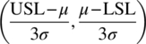 |
If lower and upper specifications are set, but only the distance from the closest limit is of relevance |
| Cpm | 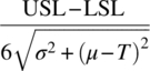 |
If a target value (T) is the desired mean operating state, Cpm adjusts the mean value to reflect the deviation from target |
| Cpu | If only a USL is required | |
| Cpl | If only a LSL is required |
In general, a process capability less than 1 describes an unacceptable system, where normal common cause variability will routinely result in failed specifications. The process is considered not capable of meeting that specification. A process with measured capability greater than 1 is considered capable of routinely meeting specifications, but in practice a process capability greater than 1.33 is often desirable so that small changes in the state of the process will not result in the process becoming incapable of achieving specifications.
41.2.4 Process Robustness During Development
During process development, it is desirable to understand process robustness even though the number of batches will be small and most batches will be run on a scale inappropriate to manufacturing. Metrics of robustness during development tend to be experimentally defined, with projection of process variability being based on expected performance given controlled process ranges. The key objective during development is to answer the question: “what range of known process parameters is acceptable to achieve product quality?”
Due to insufficient historical data of a process, models for the behavior of the new process are developed on a small laboratory scale, and inferences from those models are generalized to larger scales. Verification of those models comes only during relatively rare scale‐up campaigns to deliver DS for clinical supplies and/or drug product development. Variability is assumed by understanding plant capabilities and getting feedback from commercial manufacturing sites.
41.3 REGULATORY REQUIREMENTS FOR PROCESS ROBUSTNESS
41.3.1 Guidelines for Process Development and Validation
The International Conference on Harmonization (ICH) development and validation guidelines [ICH Q7–Q11] describe various means to help companies improve the transition from development to commercial and assure that the drug product will be manufactured fit for its intended use. In the ICH quality framework, quality, safety, and efficacy are designed into the product, and each step of a manufacturing process is controlled to assure that the finished product meets all specified quality attributes [6].
A common approach to develop a well‐understood process, designed to integrate quality, is to identify critical quality attributes (CQAs) associated with desired product quality and create predictive mathematical models that quantify the relationship between the various process parameters and the product CQAs. The models are subsequently used to define a design space: a range of process parameters that ensures the quality attributes will meet desired quantitative criteria (typically defined as ranges of acceptability, limit values, or specifications). This goal of QbD requires more fundamental understanding and modeling compared with the more conventional quality‐by‐control approach that is taken by control charts.
In parallel to this quantification, precise analytical methods to measure the CQA and other important attributes are also developed. Careful selection of process parameters during development leads to the largest possible sets of tolerable process conditions to produce high quality materials, fit for the intended purposes. There is confidence (based on experience or scale testing) that the final process based on this design space will perform consistently in the commercial manufacturing facility. Furthermore, specifications put in place for an appropriate CQA ensure that the product will have the predicted quality. All this process performance is managed in manufacturing by the Monitoring and Control Plan defined for the process.
Processes designed in the rigorous way described by the ICH guidelines usually transfer well into a manufacturing environment and deliver the expected target behavior. However, a precise estimation of the anticipated variability under manufacturing conditions is not directly accessible from development work for several reasons. Primarily, the limited development experience does not provide sufficient samples to understand the true process variability. In addition, the differences in process control are not well understood between development and manufacturing equipment trains, and there is likely more variability in manufacturing process control. Finally, the manufacturing analytical measurements often have more variability than in the development environment. This process variability is not predicted in the design space because the design space analysis and resulting unit operation models are designed to predict average process behavior. Not understanding the expected process variability, rather than just the average process behavior, may lead a development scientist to conclude that a process is robust when, in fact, there is a risk of process failure within the design space.
In order to best incorporate variability into the assessment of process robustness, we turn to a branch of statistics known as Bayesian statistical modeling. In contrast to frequentist statistics that are more commonly used in process control literature, Bayesian approaches utilize prior knowledge and limited data to estimate the plausible behavior of a process. To address the ICH guidance on design space, a Bayesian approach to understanding uncertainty has been used [7–9] not only to describe limits of failures for parameter ranges but also to more accurately map failure probability given a model and data. An advantage of the Bayesian approach over frequentist approaches is that Bayesian analysis more intuitively incorporates past observations when estimating the likelihood of unknown events and is therefore more aligned with the ICH guidance. By applying this flexible approach to determining manufacturing process capability, we aim to develop more informed and accurate models for variability while avoiding many assumptions used in standard control charts.
41.4 MODELING PROCESS ROBUSTNESS
41.4.1 Robustness of Pharmaceutical Processes
The manufacturing process for the DS may be abstracted as a mathematical relationship between the process inputs (parameters and quality descriptors of the input materials) and the process outputs, i.e. the yield and qualitative properties of the DS. This abstraction may be represented by Figure 41.2 as a mathematical function that converts inputs such as process or equipment settings into quality attribute outputs. The manufacturing process could consist of a series of unit operations incorporating chemical transformations, extractions, and isolations in the DS manufacturing process.
FIGURE 41.2 Abstract representation of a pharmaceutical process (lab: experiment or manufacturing process) where y denotes all the quality attributes of the drug substance and x the input parameters.
Typically, it is impossible to operate a process in separate instances (batch) or over time (continuous processing) under identical and/or invariant settings. Under any realistic control scheme, the input parameters will fluctuate around a target set point.
In this context, the robustness of a process may be defined as the lack of sensitivity of the process outputs, such as quality attributes, to fluctuations in the process inputs. Figure 41.3 shows a schematic of a process operated at three different target locations of the single process parameter with the same parameter variability (locations A, B, and C, in the x‐axis). The resulting distribution has a lower measure of variability in the location B, since in this region the function is less sensitive to variation in the input X. In this context the process is said to be more robust for condition B than for A or C. The input and output distributions use arbitrary units for probability density but show how identical variabilities in the inputs map to different output distributions, depending on the nature of the underlying process model. A sharp output distribution indicates that the process is robust at that input condition. In this example, operating at condition B appears to be much better than at A or C.
FIGURE 41.3 Sensitivity of the output (y) to a given variability in the input (x) at different locations of the process input parameters.
In the example above, the source of variability (and corresponding process robustness) was restricted to variability in the input parameters. However, a given measure of the quality of the pharmaceutical product (potency, purity, etc.) will also be subjected to the intrinsic process equipment variability as well as measurement or analytical variability. These additional sources need to be incorporated to determine a comprehensive analysis of the process variability for a given outcome and the corresponding relevant process robustness. Figure 41.4 shows a process with the same input parameter sensitivity but with an additional measure of process variability using random error with a relative standard deviation of 5%. The output distribution is now affected by both the input distribution on the model and the random process variability.

FIGURE 41.4 Output variability in a process with random variation in addition to input variability.
In comparing Figures 41.3 and 41.4, it is evident that the inputs that lead to optimal robustness are different than if we only considered the mean response from the model. The extra noise incorporated into the robustness assessment means that input condition A now has a narrower output distribution than condition B or C. The general approach to characterize process robustness is to measure the process outcome as a function of the process inputs and build a model that estimates the mean of the observed outcome, i.e. a causal model. Subsequently the probability of a given observation deviating from the model is estimated by constructing a model for the process that takes this uncertainty into account.
The established view of process variability (the random distribution around the mean value) is that it is generated from random fluctuations of variables that are not necessarily accounted for in the process description. To the extent that a source of variability can be understood, quantified, and included in the causal model as an input variable, the robustness of the process can be improved by adding control over that variability source (a causal input).
The next sections will discuss general procedures to determine, evaluate, and control process variability in the context of process robustness optimization.
41.5 PROCESS UNCERTAINTY
41.5.1 A Manufacturing Process as a Random Number Generator
The general practice in chemical engineering pharmaceutical development is to represent relevant unit operations involved in the manufacturing as mathematical models that provide a quantitative relationship between the control variables and the quality attributes, which may be represented by Eq. (41.3):
where, in this case,
- f(…) represents the structure of the model.
- x and θ are the process inputs of the control variables and model parameters.
- y represents the quality‐relevant attributes that are impacted by the unit operation, i.e. the CQAs of a pharmaceutical process.
Although relationships of this form are generally used in developing a design space and a corresponding control strategy, it should be recognized that under standard regression techniques, the predictions will represent estimates only of the expected mean response from the unit operation, not the risk of deviations.
Rather than expressing the model uncertainty as an error, the formalism implemented in this chapter aims to describe the estimate of the process outcome y as a probability of possible outcomes. Instead of single values or expected outcomes, inputs and outputs can be considered as probability distribution functions (PDFs) where values have some likelihood of occurrence. We consider the physical (and chemical) process of manufacture and measurement of the QAs as a physical random number generator (RNG). The goal is then to generate a probabilistic model that incorporates the causal relationships determined from the underlying physicochemical nature of the process or an empirical observation of correlation between y and the x vector and a stochastic contribution from the inherent variability of the process and the measurement. The model then incorporates both a causal part (f parametrized by θ) and a stochastic part (parametrized by τ). In practice, we wish to define a RNG whose distribution closely simulates the observable quantity of interest, i.e. instead of a conventional use of a model, we will redefine our model as a PDF (Eq. 41.4):
Equation (41.4) describes predicted quality attributes (y) as being a random sample taken from a PDF that depends on operating conditions (x), causal (θ) parameters, and stochastic (τ) parameters. This approach is an attempt to capture the impact of our ignorance on the exact ability to predict and measure y, which manifests itself as uncertainty.
The formalism requires incorporation of causal and stochastic compartments in the model. The causal part is the conventional model structure (mechanistic or empirical) that is conventionally used. The stochastic part requires incorporation of a hypothesis of uncertainty propagation in the process and may also include uncertainty in the control parameters encoded in the vector x.
The result is a multidimensional probability distribution (the posterior) of all the parameters in the model. Bayesian inference methodology to estimate the model parameters has been described in Albrecht [10] and Gelman [11]. This distribution of parameters can then be used to obtain the PDF of future observations from Eq. (41.3), using the posterior parameters inferred from Eq. (41.4). Specifically the methodology results in the definition of an RNG whose distribution best describes the data that was sampled from the physical RNG that we are attempting to understand.
Therefore, the process of estimating the model (causal and stochastic) parameters provides a framework to estimate the PDF of future observations (ypred). Ultimately, we estimate the probability of y given x, conditional on prior observations of the relationship of y to x (the data) under a postulated mathematical relationship (the model) that is a function of model parameters θ and observational noise τ. Each of these three groups of values has their own types of uncertainty.
Later in this chapter, we describe a methodology to build RNGs for pharmaceutical development applications by incorporating Bayesian framework. A model is developed to predict the quality attribute of interest. The process variability is simulated by incorporating the variability of the input process parameters, model uncertainty, and analytical (measurement) variability. These models were incorporated and simulated using Stan [12] from the RStan package available in R [13]. This approach allows great flexibility in proposing and testing new model structures, both to best develop models not only for the process and to describe the sources and distributions of process, model, and measurement errors. Hierarchical models to describe the common and individual errors could therefore be used to describe inter‐ and intra‐lot measurement variability. Once the RNG is developed based on available experimental data, it is subsequently used to sample the distribution of potential outcomes in the commercial manufacturing environment.
41.5.2 Variability from Process Parameters and Inputs/Control Parameter Variability
During pharmaceutical manufacturing, there are many potential causes of variability due to the relative complexity and uniqueness of each processing step and the difficulties in perfect control during batch processing. Most commonly, variability arises from the failure to perfectly achieve target parameter states. Much of this variability is expected and should be accommodated by robust manufacturing processes. Material charges, such as reagents, solvents, and catalysts, may not be exactly as expected due to errors in weighing or material hang up during the charging procedure. Temperature may not be controlled exactly as specified due to drifts in thermocouple calibrations, inability for reactor jackets to cool against exothermal events, controller oscillation, or many other reasons. These variations are usually mild and do not cause process failure, but the result is a process that displays significant common cause variability during normal manufacturing conditions. Drifts in manufacturing equipment may also cause process variability, due to slow but steady breakdown in the operating condition of any particular equipment train. This equipment is periodically adjusted through calibration or scheduled maintenance, causing variability in the processing conditions but not outright failure. Equipment may also be replaced, or the process may be shifted to new equipment, causing many slight differences in processing conditions that may not be easy to identify when taken in total with all common cause variability.
Input material quality fluctuations can cause process variability if the quality attributes of the product depend on the quality attributes of the input material. Sometimes, impurities from inputs are directly present in output product, causing a chain of process variability that cascades down the synthetic sequence. Alternately, attributes of the input material like water content, residual solvent, residual acid/base, or inorganic salt content can affect the process responses of an output in a way that increases process variability. For example, an organic solvent like acetone may have variable water content depending on the source or batch used on a particular day. This water variability (potentially measured in ppm) may cause a water‐sensitive reaction to behave slightly differently. This difference in behavior may lead to a slight increase in impurity level, so the variability in measured impurity level becomes dependent on the source and batch of acetone used in the reaction, which may change over time.
41.5.3 Model Uncertainty/Epistemic Uncertainty
In quantifying uncertainty for process models, the term epistemic uncertainty describes uncertainty that is due to insufficient knowledge of a system. Process input variability was described in the previous section and described the contribution of variability in the value of x from Eq. (41.4). Epistemic uncertainty stems from a lack of knowledge of some “ground truth,” such as a regressed model parameter θ in Eq. (41.4). By increasing the amount of data and analysis, the uncertainty of these parameters will shrink until only the true value can be considered possible. Examples of epistemic uncertainty include confidence intervals for regression, as well as the relative confidence in the ability of different models to describe a set of data. Often, the assumption that the model structure is appropriate must be examined. This can be performed by assessing the performance of a family of potential models though approaches such as stepwise regression [14] or by performing experiments that best discriminate among models [15].
41.5.4 Observational Variability/Aleatory Variability
Aleatory variability is defined as an uncontrollable random effect, such as a game of chance that produces a random outcome where the degree of risk can be known in advance. The overall probability distribution of aleatory variability can be knowable, but any single observation of a system that is subject to aleatory variability cannot be predicted exactly. Even with a large number of identically prepared samples, the observed values will vary. Aleatory variability occurs at each step in the sampling collection, analysis, and reporting. For example, even on a calibrated analytical instrument, a reference standard will have some observed variability in measurement due to the inherent precision of the machine. The resulting signal over many repeated measurements will average to the true reference value, despite the noise in the individual measurements. Analytical equipment used in the pharmaceutical industry typically has a high signal‐to‐noise ratio to reduce this source of aleatory variability, but there are other sources. A common problem arises in sampling from a heterogeneous mixture. Such samples will have variability in their analysis, but as more samples are taken, the average of the samples will become closer to the true value. While aleatory variability can only be reduced with changes to sample collection and analysis, its contribution to the overall uncertainty in ypred can be estimated from data. For simple linear models, approaches such as analysis of variance (ANOVA) [14] are commonly used to estimate the contribution of τ in Eq. (41.4). For nonlinear models that are relevant to the fundamental mechanics of a system, Bayesian approaches are recommended to most accurately separate epistemic uncertainty from parametric and aleatory variability.
41.6 BRIEF OVERVIEW OF PROBABILISTIC GRAPHICAL MODELS
41.6.1 Background and Core Concepts
Probabilistic graphical models (PGMs) are a powerful framework to define probabilistic analysis problems [16]. This formalism allows for definition of a large variety of problem statements while also enabling rigorous solution methods for that problem. They are a simple visual tool to define problem statements according to some basic rules, but a problem that can be defined by a PGM can be solved using a suite of specialized mathematical algorithms such as those outlined in the next section. PGMs represent uncertain probabilities as oval nodes connected by arrows that represent causal influence. Many problems can be formulated by a subset of as PGMs known as directed acyclic graphs (DAGs). In a series of nodes connected by directional arrows, the acyclic constraint of DAGs forbids a loop around a group of nodes. Arrows between nodes define the direction of causality of how one node influences the value of another. While the nature of that influence is not explicitly labeled in the graph, it must be accounted for when formulating and computing the model. Of the many solution methods that exist, Markov chain Monte Carlo (MCMC) (Section 41.6.3) will be presented as the preferred solution algorithm for the types of problems experienced during process development.
In this chapter, uncertainty is considered in the probabilistic sense of a value existing within a probability distribution. In using models for process robustness, there are two phases: first quantifying the uncertainty of a process given any available data or fundamental knowledge and then applying the degree of uncertainty to make future projections of robustness. The previous Sections 41.5.3 and 41.5.4 described the sources and nature of epistemic and aleatory variability. Both types of uncertainties will be considered in the modeling of process robustness using PGMs.
41.6.2 Hierarchical Models
The term hierarchical models, while not formally defined, typically refers to model with multiple layers of complexity relating inputs to outputs. For process models, the hierarchy starts with uncertain process inputs followed by uncertain model predictions, followed by observational errors. Variability in CQA measurements can be likewise described as contributions stemming from analyst, equipment, and intra‐lot and inter‐lot variability components. Figure 41.5 shows an example of measuring the composition of a heterogeneous batch, factoring in variability in collecting samples and measurement error.
FIGURE 41.5 Hierarchical graphical model example for analyzing a heterogeneous batch for content uniformity.
In Figure 41.5, the observed composition for any sample depends on the true sample composition that in turn depends on the true batch composition. Noise associated with batch sampling variability and analysis variability together influence any measurements of composition. While the batch and sample compositions have a single ground truth value, the aleatory variability introduced by the process of gathering a sample and the sample analysis will cause the observed composition to vary. With only composition observation from multiple analyses, it is possible to determine the true value of the sample and batch composition (within a range of epistemic uncertainty). The variability in the observations can be separated into the contributions from the aleatory variability of the sampling and analysis process to identify the remaining epistemic uncertainty of the batch composition. This degree of confidence in our knowledge of the underlying truth is needed to provide a proper accounting of robustness and risks.
41.6.3 Capturing Uncertainty with Markov Chain Monte Carlo
With MCMC, any computational model with uncertain parameters can have the probability distributions of those parameters be fully estimated. MCMC can be conceptualized as a series of random jumps or hops (called a Markov chain) between possible parameter values. Each hop represents a set of model parameter values that are randomly selected from a distribution. Using these parameters, the model is used to make predictions of the observations. These predictions are compared with the observed values and the goodness of fit is assessed. As with regular Monte Carlo, samples are drawn from a random distribution, but with MCMC, the performance of each set of samples is compared with the performance from the previous iteration. Combinations of model parameters that better describe the observations are identified, and the MCMC algorithm is more likely to use similar values for future hops. As the number of hops between states becomes very large, the resulting distribution of parameter values, called the posterior distribution, begins to approximate the true parameter value distribution. MCMC approaches, while computationally expensive, are essential tools to estimate parameter uncertainty ranges for models with non‐normally distributed errors or with nonlinear models [10].
The output of an MCMC simulation is a list of typically thousands of posterior samples of the uncertain parameters. Each sample contains a self‐consistent set of parameters that is credible given the data and underlying model. Combinations of parameters that do a better job of predicting the observations will appear more frequently in this list, and less likely combinations of parameters will appear less often. By plotting histograms of the individual parameters, summary statistics such as mean and standard deviation of model parameters can be calculated. By plotting 2D histograms of two parameters, joint probabilities can be visualized. This approach can be used to quickly understand correlations between modeled parameters. The samples from the parameter posterior distributions represent all credible combinations of regressed parameter values; any estimation of model robustness must use these samples to properly account for uncertainty in predicted outcomes.
For a simple example of MCMC, consider a simple nonlinear equation in Eq. (41.5), where a result, y, is a function of input x, determined by parameters a and b:
Data is collected for y with a = 1 and b = 0.5, with normally distributed error with a standard deviation of 0.1 added, shown in Table 41.3.
TABLE 41.3 Example Data for Parameter Regression
| x | y True | y Observed |
| 1 | 2.00 | 1.90 |
| 2 | 2.41 | 2.49 |
| 3 | 2.73 | 2.67 |
| 4 | 3.00 | 3.20 |
| 5 | 3.24 | 3.34 |
| 6 | 3.45 | 3.55 |
| 7 | 3.65 | 3.65 |
| 8 | 3.83 | 3.90 |
| 9 | 4.00 | 4.06 |
| 10 | 4.16 | 4.25 |
In the observed data, underlying true model and MCMC results are plotted in Figure 41.6.
FIGURE 41.6 Regression using MCMC.
In Figure 41.6, the MCMC results are plotted as family of faint prediction trends, one trend from each of the posterior samples of a and b. In aggregate, the prediction trends describe the data well and are in agreement with the ground truth model. The distribution of these parameters and their correlation are plotted in Figure 41.7. From MCMC, the most likely values for a and b (1.01 and 0.51, respectively) are very close to their true values. This pairwise plot shows the distribution of a and b along the diagonal, the correlation coefficient (upper right), and joint probability contours (lower left) of a vs. b.
FIGURE 41.7 Correlation between parameters regressed by MCMC.
The negative correlation between a and b is important to carry forward when using the model to make robustness predictions. Focusing only on the individual distributions of the regressed parameters makes the mistake of implying that they are independent, contrary to what the MCMC regression has shown. If one parameter is at the upper end of its distribution, the other must be near the low end of its distribution to make credible predictions. While conventional nonlinear regression approaches using a frequentist approach to statistics [17] can calculate parameter covariance, there is the underlying assumption of linear behavior near the optimal parameter values. Only Bayesian approaches such as MCMC can determine the full joint probability distributions needed for an accurate assessment of robustness and the likelihood of rare events.
41.6.4 Utilizing Uncertainty for Process Robustness
Once the epistemic uncertainty of the model parameters is characterized by MCMC, the model can be applied to any scenario where the process has some degree of aleatory variability. This involves utilizing each sample of the MCMC posterior with a simple Monte Carlo simulation. The resulting values combine the process variability with the epistemic uncertainty of the process model. From these values, forecastable metrics such as failure rate and Cpk can be calculated. This two‐step process of regressing model parameters using MCMC followed by using the parameter uncertainty to predict a range of probable future outcomes using Monte Carlo is illustrated in Figure 41.8.

FIGURE 41.8 Workflow to convert a model and data to a prediction range while preserving uncertainty.
41.7 SIMULATION TOOLS FOR BAYESIAN STATISTICS
Modeling uncertainty is a persistent challenge, especially for nonlinear models. Typical approaches such as confidence intervals cannot be accurately applied to nonlinear models and to models where the sources of noise are not uniform. Fortunately, Bayesian statistical inference is now easier than ever, thanks to modern computational approaches [11]. With the growing advances, it is now possible to compute even large hierarchical models with hundreds or thousands of variables. MCMC is an essential tool in estimating uncertainty for complex systems. MCMC approaches have been recently recognized within the chemical engineering community as being well suited to pharmaceutical process modeling as they can incorporate expert judgment with sparse data sets to yield estimates of risk in a manner consistent with regulatory guidance [7, 18]. The interpretability and communication of the results becomes more straightforward, as the confidence intervals from frequentist statistics unnaturally describe the range of conclusions expected over many replicated studies. By contrast, Bayesian credible intervals more intuitively describe the likelihood that a parameter truly has a given value. By avoiding the some of the assumptions used in frequentist statistics, this approach can more accurately estimate the intervals of parameters regressed using nonlinear regression [10, 18].
41.7.1 Overview of Available Software Tools
Basic versions of the MCMC algorithm are straightforward to program [19]; therefore, implementations can and do exist in many programming languages. However, as more sophisticated and computationally efficient approaches are developed, using a MCMC library maintained by a third party enables more rapid setup and execution of a simulation. A recent (2017) list of these packages used by the statistics and modeling communities includes Stan [12], WinBUGS [20], PyMC3 [21], and Emcee [22].
Because the selection of software is highly dependent on the end user's circumstances and need, a deeper assessment of each of these tools is left to the individual user. Attributes to keep in mind when selecting a software package include setup time and cost, available documentation, and available algorithms. In this section and the following section, Stan was selected due to its availability as an open‐source program, refined interface with R via RStan [13], and portability of Stan models between other programming languages.
41.7.2 Model Diagnostics
Assessing the quality of the modeling is an important check against implementation errors and poorly specified models. MCMC simulations in particular have two main challenges to performance [23]: convergence and autocorrelation. Checks of these performance measures should be done to ensure that the MCMC results are valid and can be used for predicting process robustness.
41.7.2.1 Convergence
A common problem with MCMC is a lack of convergence of the Markov chains, resulting in an incomplete coverage of parameter space. This is equivalent to local minima in an optimization problem. Fortunately, there are many approaches to prevent and identify when a MCMC chain does not converge. The most common approach is to run multiple chains simultaneously in parallel and to ensure the chains reach a consensus distribution. A warm‐up (sometimes called burn‐in) period of several thousand iterations is also used to ensure that the chains have enough time to move from their random starting points to their final distribution and that they are in agreement. This consensus can be visualized by plotting the distribution of chains over time or assessed statistically with metrics such as potential scale reduction factor [23]. For a basic visual check, make sure that the multiple chains overlap (mix) and that there is no overall drift in the distribution as the simulation is run. Figure 41.9 shows the trace of the Markov chains from the example in Section 41.6.3. The chains show no long‐term trends and are in good agreement, indicating convergence. The values for each parameter are equal to 1, indicating ideal performance.
FIGURE 41.9 Markov chains at each iteration of the simulation described in Section 41.6.3.
41.7.2.2 Autocorrelation
Other issues related to MCMC are due to autoregression in the sampling. Autoregression occurs when the sampling is inefficient, causing the Markov chain to slowly converge to the final posterior distribution. This causes the individual parameter samples to remain unchanged over several Monte Carlo iterations, distorting the posterior distribution. Sample thinning is an approach that reduces the overall number of samples by keeping only a subset (such as every 10th or every 50th sample) of the posterior samples. The degree of thinning increases the accuracy of the posterior distribution, but because many iterations are discarded from the analysis, there is a trade‐off of wasted computation time. Figure 41.10 shows the autocorrelation of the Markov chains from the example in Section 41.6.3. For each bar plot panel, the autocorrelation at a lag 0 is always 1 (a sample is perfectly correlated with itself). After one random sampling iteration, the sampled parameter value is approximately 50% correlated with the previous sample for both parameters a and b in each chain. This correlation across samples introduces biases in any subsequent analysis. As the chain is iterated, the autocorrelation eventually drops to near 0. In Figure 41.10, the autocorrelation after a lag of 10 iterations is roughly zero. This means that the chain should be thinned by only keeping every 10th sample to ensure that each sample is independent. Plotting the chains after this thinning step would show a plot with a value of 1 at lag 0 but nearly zero correlation for all other values of lag.

FIGURE 41.10 Plots of autocorrelation for parameter regression for parameters a and b in Chain 1 and Chain 2.
41.8 EXAMPLE OF MODELING PROCESS ROBUSTNESS
An example calculation of process robustness will be presented in this section. The goal of this example is to present scenarios similar to real situations in which MCMC has been applied to inform decision makers during pharmaceutical process development. The goal in the example is to assess process robustness of a crystallization operation at a larger scale, accounting for the uncertain model and uncertain inputs. The example will use R and Stan [13] to analyze the raw data, regress the model, and determine the uncertainty of the outcome under different conditions.
41.8.1 Problem Statement
In this example, a crystallization process follows an empirical model under uncertain operating conditions. Here, the batch process will be run at a facility that has a known distribution of process control. The final crystals must have a particle size (D90) of 100 ± 30 μm. Some experiments have been conducted on a different scale to collect data to build a model. Table 41.4 shows a set of DoE data collected at the lab scale to develop a crystallization model. At each condition, three physical samples were each analyzed twice to understand the sources of sample collection heterogeneity and analytical error. These steps introduce errors that confound the regression of the model parameters.
TABLE 41.4 Crystallization Data
| Scale | T | X | D90 Sample 1 Analysis 1 | D90 Sample 2 Analysis 1 | D90 Sample 3 Analysis 1 | D90 Sample 1 Analysis 2 | D90 Sample 2 Analysis 2 | D90 Sample 3 Analysis 2 |
| Lab | 40.0 | 5.0 | 93.2 | 100.1 | 94.1 | 91.7 | 93.9 | 93.7 |
| Lab | 40.0 | 10.0 | 85.2 | 75.4 | 76.1 | 81.9 | 76.0 | 69.2 |
| Lab | 40.0 | 15.0 | 69.6 | 73.2 | 69.8 | 66.1 | 77.4 | 73.9 |
| Lab | 50.0 | 5.0 | 131.9 | 117.5 | 1.2 | 134.1 | 120.5 | 126.4 |
| Lab | 50.0 | 10.0 | 117.0 | 98.3 | 103.1 | 116.4 | 96.9 | 98.0 |
| Lab | 50.0 | 15.0 | 104.7 | 87.9 | 90.9 | 97.6 | 82.1 | 86.5 |
| Lab | 60.0 | 5.0 | 143.8 | 153.6 | 137.4 | 150.8 | 155.0 | 4.0 |
| Lab | 60.0 | 10.0 | 127.2 | 128.4 | 125.9 | 135.0 | 122.0 | 122.4 |
| Lab | 60.0 | 15.0 | 116.4 | 108.0 | 105.8 | 116.9 | 116.5 | 119.0 |
41.8.2 Process Model Definition
The desired empirical model describes a linear relationship between the particle size (expected D90), seed temperature T, and cooling rate X:
With the model in Eq. (41.6), the goal is to determine the likelihood that the variability in process inputs will cause the product to be out of specification. This will in turn determine the distribution of Cpk that will be expected at a manufacturing scale. The model for expected D90 is purely deterministic, so no variability is expected between batches with constant operating conditions; however, we know that there will be some random variability in sampling and in sample analysis. Because the batch may have some intrinsic heterogeneity, Eq. (41.7) models the sampling variability as a normally distributed multiple of the expected D90:
Likewise, repeated analysis of the same sample is expected to result in some variability of the measurement. Equation (41.8) adds a similar error source as in Eq. (41.7) to the batch sample:
To add more complexity to the problem of estimating the model parameters, the degree of sampling and measurement variability σsamp and σmeas are assumed to be unknown in the fitting exercise.
The model definition and errors due to sampling and analysis can be summarized by the PGM in Figure 41.11.
FIGURE 41.11 Crystallization robustness described as a probabilistic graphical model.
In the PGM in Figure 41.11, the boxes represent a stacking of separate nodes for each of the replicates; in this case there will be nine nodes each for expected batch D90, T, and X to represent the individual experiments. There will be 27 (3 × 9) sample D90 nodes for each sample and experiment and 54 (2 × 3 × 9) observed D90 nodes for each analysis of each sample at each experimental condition.
41.8.3 Estimating Uncertainty
The data in Table 41.4 can be fit simultaneously to Eq. (41.8) using Stan while capturing hierarchical sources of error stemming from measurement and prediction errors. Here the MCMC routine uses 15 000 iterations with two chains, for a total of 30 000 samples. Convergence is assessed by manually examining the chains as well as the conversion statistics ![]() . In this case, convergence and autocorrelation measures confirmed that the simulation was successful.
. In this case, convergence and autocorrelation measures confirmed that the simulation was successful.
The distribution of the regressed parameters is shown in Figure 41.12, showing that there is some covariance between the A and B model parameters but that the other pairs of parameters are independent distributions.
FIGURE 41.12 Regressed model parameters.
The MCMC routine works well to separate and quantify the sources of the uncertainty in observed D90. Table 41.5 shows the parameter values estimated by MCMC. The true value of the parameter (used to generate the data in Table 41.4) is compared to the mean and standard deviation to confirm that the MCMC model can recapture the true model parameters within the 95% interval of its estimates. In the case of this model, the larger CV for the model parameters A, B, and C relative to the magnitude of the sampling and measurement variability indicates that much of the uncertainty is due to epistemic uncertainty; therefore more experimental data will increase the model confidence and therefore prediction accuracy.
TABLE 41.5 Parameter Values Estimated from MCMC
| Parameter | Parameter Mean | Parameter Standard Deviation | True Value |
| A | 12.17 | 6.57 | 20 |
| B | 2.41 | 0.13 | 2.2 |
| C | −2.68 | 0.29 | −2.5 |
| σsamp | 0.06 | 0.01 | 0.05 |
| σmeas | 0.04 | 0.01 | 0.05 |
The next step is to determine the optimal operating conditions to minimize variability. Because the model equation is simple, an algebraic approach can be used here. Using distributions of the parameters A, B, and C, the optimal values for T and X to meet the target D90 of 100 μm can be determined to satisfy Eq. (41.9):
Scanning across a range of X, the corresponding values of T can be calculated from the regressed parameters, and the model credibility can be estimated from the posterior samples. Figure 41.13 plots the combination of X and T values that are expected to result in a D90 of 100 μm. While any point along the line is expected to meet this target, the uncertainty of the model can also be incorporated to find conditions where the model is more confident. The optimal value of X to minimize variability due to epistemic uncertainty (thinnest region of the uncertainty band in Figure 41.13) of the model parameters corresponds to approximately X = 10, T = 48. These are the best conditions to use in order to maximize manufacturing robustness.
FIGURE 41.13 Combinations of inputs X and T to meet product specifications, with a range of uncertainty.
41.8.4 Robustness Predictions
With the regressed model and posterior samples, the next step is forecasting the risk of generating batches that exceed the particle size specification. Using the terminology from Section 41.5.3, the posterior distribution from MCMC contains the epistemic uncertainty of the parameters; resampling from these results and using the aleatory variability in a manufacturing facility will forecast the CQA variability. This approach allows for an arbitrary posterior distribution and a more accurate representation of the true model error under different circumstances. In this example, we suppose that an independent study determines that the nucleation temperature T and cooling rate X in manufacturing is controlled to be within 5 °C and 0.5 °C/h, respectively, 99% of the time, following a normal distribution. The analytical variability σmeas is also independently determined to be 5%. Now with these sources of aleatory variability, the risk of exceeding the particle size specification can be calculated from the posterior distribution.
Using these ranges, the model described in Figure 41.11 is run using MCMC to calculate the distributions of the model parameters. These posterior distributions for the parameters are then resampled using Monte Carlo to calculate the range of future observed D90 values and the corresponding values for the Cpk. Random samples for X and T are taken from their distributions and used; next, random noise is added. These model outputs are plotted as histograms in Figure 41.14. Here, the Cpk we expect to observe in manufacturing may be between 0.75 and 1.25 but is most likely to be near 1.
FIGURE 41.14 Future predictions of D90 at manufacturing.
Additionally from the distribution of D90, the empirical cumulative distribution function (ECDF) can be used to determine the likelihood of observing a D90 value below a certain specification. The ECDF is simply the cumulative integral of the probability distribution calculated by Monte Carlo and is used to determine the proportion of outcomes that are below a given value. Table 41.6 highlights how the likelihood of the process meeting a specification changes as the USL is increased. For example, a specification of 100 μm would be near the average expected D90, so the chance of meeting that specification would be approximately 50%.
TABLE 41.6 Empirical Cumulative Distribution Function Values from Expected Range of D90
| D90 Upper Specification Limit | Expected Chance of Observing D90 Below Specification Limit (%) |
| 80 | 0.4 |
| 90 | 8.0 |
| 100 | 45.4 |
| 110 | 86.9 |
| 120 | 98.8 |
This type of analysis also allows for teams to quickly asses the quality manufacturing predictions as new batches are run. For example, if a batch had an observed D90 of 90 μm, this difference from the expected D90 could be within normal variability, as there is a predicted 8% (or 1 in 12) chance of this occurring. Such a difference may not warrant immediate intervention. However, if a batch has an observed D90 of 80 μm, the much lower likelihood (1 in 250) of this occurrence would strongly suggest to the team that process is not performing consistently with the model built from the lab experiments and should be investigated further to identify a cause.
SUMMARY
In summary, pharmaceutical process development is uniquely sensitive to variability due to the common use of batch processing, relatively sparse process knowledge, time constraints, and high process complexity. Models for process robustness are becoming an essential tool for process development thanks to the triple convergence of business needs for faster development times, computing hardware, and publicly available software to lower the barrier to apply these approaches. Such approaches now enable the estimation of the process capability to expect in any manufacturing facility, greatly facilitating technology transfer activities. While the recent and ongoing advances in robustness assessment enable more quantitative assessments of pharmaceutical quality prediction, there is no substitute for an engineer's expert judgment and critical thinking. To maximize the process robustness under a given set of constraints, the control strategy, process sensitivity, process variability, and selection of quality limits are all important considerations. This chapter demonstrates that by embracing a probability mind‐set, powerful statistical tools can enable a rational, quantitative assessment of risk.
SUPPORTING INFORMATION
The source code used to create the example data, probabilistic models, and figures are available as a Jupyter notebook (jupyter.org) at DOI: 10.6084/m9.figshare.7607354. The supporting information also includes version numbers and installation instructions for the programming language R and associated function libraries.
REFERENCES
- 1. Anderson, D.R., Sweeney, D.J., Williams, T.A. et al. (2010). Statistics for Business and Economics. Independence, KY: South‐Western CENGAGE Learning.
- 2. Reid, R.D. and Sanders, N.R. (2011). Operations Management: An Integrated Approach, 4e. Hoboken, NJ: Wiley.
- 3. NIST/SEMATECH (2013). NIST/SEMATECH e‐Handbook of Statistical Methods. http://www.itl.nist.gov/div898/handbook (accessed 4 April 2018).
- 4. Nomikos, P. and MacGregor, J.F. (1995). Multivariate SPC charts for monitoring batch processes. Technometrics 37 (1): 41–59.
- 5. Anderson, T.W. (2003). An Introduction to Multivariate Statistical Analysis. New York: Wiley.
- 6. ICH (2011). ICH‐endorsed guide for ICH Q8/Q9/Q10 implementation. ICH Quality Implementation Work Group Points to Consider (R2) (accessed 4 April 2018).
- 7. Peterson, J.J. (2008). A Bayesian approach to the ICH Q8 definition of design space. Journal of Biopharmaceutical Statistics 18 (5): 959–975.
- 8. Peterson, J.J. (2010). Design space and QbD: It's all about the (stochastic) distributions. AIChE Annual Meeting, Conference Proceedings, Salt Lake City, UT (7–12 November 2010).
- 9. Tabora, J.E. and Domagalski, N. (2017). Multivariate analysis and statistics in pharmaceutical process research and development. Annual Review of Chemical and Biomolecular Engineering 8: 403–426.
- 10. Albrecht, J. (2013). Estimating reaction model parameter uncertainty with Markov Chain Monte Carlo. Computers and Chemical Engineering 48: 14–28.
- 11. Gelman, A., Carlin, J.B., Stern, H.S. et al. (2013). Bayesian Data Analysis, 3e. Boca Raton, FL: Taylor & Francis.
- 12. Stan Development Team (2016). Stan modeling language users guide and reference manual, version 2.14.0.
- 13. Stan Development Team (2016). RStan: the R interface to Stan, R package version 2.14.1.
- 14. Kutner, M.H., Nachtsheim, C.J., and Neter, J. (2003). Applied Linear Regression Models. New York: McGraw‐Hill.
- 15. Box, G.E.P. and Hill, W.J. (1967). Discrimination among mechanistic models. Technometrics 9 (1): 57–71.
- 16. Koller, D. and Friedman, N. (2009). Probabilistic Graphical Models: Principles and Techniques. Cambridge, MA: MIT Press.
- 17. Seber, G.A.F. and Wild, C.J. (eds.) (2005). Statistical inference. In: Nonlinear Regression, 191–269. Hoboken: Wiley.
- 18. Blau, G., Lasinski, M., Orcun, S. et al. (2008). High fidelity mathematical model building with experimental data: a Bayesian approach. Computers and Chemical Engineering 32 (4–5): 971–989.
- 19. Beers, K.J. (2007). Numerical Methods for Chemical Engineering. New York: Cambridge University Press.
- 20. Lunn, D.J., Thomas, A., Best, N., and Spiegelhalter, D. (2000). WinBUGS: A Bayesian modelling framework: concepts, structure, and extensibility. Statistics and Computing 10 (4): 325–337.
- 21. Salvatier, J., Wiecki, T.V., and Fonnesbeck, C. (2016). Probabilistic programming in Python using PyMC3. PeerJ Computer Science 2: e55.
- 22. Daniel, F.‐M., Hogg, D.W., Lang, D., and Goodman, J. (2013). emcee: The MCMC hammer. Publications of the Astronomical Society of the Pacific 125 (925): 306.
- 23. Gelman, A., Carlin, J.B., Stern, H.S., and Rubin, D.B. (2003). Bayesian Data Analysis, 2e. Boca Raton, FL: Taylor & Francis.