
19
A GENERAL FRAMEWORK FOR SOLID–LIQUID EQUILIBRIA IN PHARMACEUTICAL SYSTEMS
Thomas Lafitte, Vasileios Papaioannou, Simon Dufal, and Constantinos C. Pantelides
Process Systems Enterprise Ltd., London, UK
19.1 INTRODUCTION
A large proportion of active pharmaceutical ingredients (APIs) are produced and administered in the solid form. As a result, the thermodynamic equilibrium of systems involving solid and liquid phases is of central importance to API manufacturing where unit operations such as crystallization, particularly in organic solvents, play a prominent role in the separation and purification of APIs and their intermediates during chemical synthesis. Equilibrium compositions determine the driving forces for crystal formation and growth, and are important factors for the selection of an appropriate solvent for each separation step.
Solid–liquid equilibrium in aqueous environments also plays a central role in the oral absorption of pharmaceuticals [1], this time in determining the driving forces for dissolution of solid APIs in the lower gastrointestinal (GI) tract, consequently affecting drug bioavailability, particularly in the case of very low solubility drugs. The variation of pH along the GI tract and the presence of a variety of ions may also cause the reprecipitation of the API in various forms (e.g. salts) at different sections of the GI tract, which may have an inhibitory effect on bioavailability.
Recent years have witnessed a significant increase in the use of sophisticated mathematical models both in the design of pharmaceutical manufacturing operations and for the understanding and enhancement of oral absorption via appropriate formulations. The accurate computation of solid–liquid equilibria in mixtures of given temperature and composition is particularly important in this context as it can greatly affect the accuracy of predictions of the overall model. However, this poses a number of challenges. Some of these arise because of the complexity of the solid forms themselves. For example, acidic or basic APIs may combine with cations or anions present in the system to form salts. Crystallization in organic or aqueous media may result in solvent molecules being incorporated in the crystal structure, resulting in the formation of solvates or hydrates of fixed composition. There is also increasing interest in the use of co‐crystals [2, 3] as a means of improving the solubility of poorly soluble APIs. Moreover, in any particular system, multiple solid forms relating to the same API may exist either simultaneously or in different regions of the composition and temperature domains; and multiple crystal structures (polymorphs [4]) having the same molecular composition may exist under different conditions.
Another set of challenges arises from the potential complexity of the solvents and their interactions with the API in the liquid phase. This is particularly pronounced not only in the case of aqueous media but also in other strongly associating solvents (e.g. alcohols) involving hydrogen bonding. The use of mixed solvents, either for enhancing the solubility of a target solute or for causing its precipitation via antisolvent effects, is also widespread. Moreover, under certain conditions, multiple liquid phases may form as is the case, for example, with undesirable “oiling out” effects that result in API‐rich and API‐lean phases [5, 6]. In aqueous mixtures, further complications arise because of the presence of ions and liquid‐phase reactions such as acid/base dissociation.
This chapter presents a unified framework for the determination of solid–liquid equilibria in complex systems of the types outlined above. The framework is based on a fundamental thermodynamics formulation of the combined phase and reaction equilibrium problem (see Section 19.2), supported by the emergence, over the past decade, of new equations of state (EoS) that are capable of accurately predicting liquid‐phase behavior of mixtures involving complex intermolecular interactions (see Section 19.3).
An important consideration in the context of any modeling framework is the amount of experimental data required for the characterization of any particular system of interest in terms of the parameters required by the model. This issue is considered in detail in Section 19.4, with particular focus on the characterization of solid‐phase behavior with minimal experimental solubility data.
Section 19.5 presents several examples illustrating key aspects of the proposed framework, and Section 19.6 draws some general perspectives from these examples. Finally, Section 19.7 concludes with a summary of the presented approach.
19.2 THERMODYNAMIC FUNDAMENTALS FOR SOLUBILITY CALCULATIONS
In this section, we review the fundamental thermodynamics underpinning the computation of solubilities, to the extent necessary for understanding the overall approach presented in this chapter.
Section 19.2.1 reviews the general conditions for thermodynamic equilibrium in a multiphase multi‐reaction system. Section 19.2.2 then discusses how these general conditions can be applied to a wide class of systems of interest to the pharmaceutical industry, including those involving solid phases with API salts, hydrates or solvates, or co‐crystals. It will be seen that the only physical properties required in all cases are chemical potentials in liquid and solid phases; these are covered in Sections 19.2.3 and 19.2.4, respectively.
19.2.1 General Conditions for Phase and Reaction Equilibrium
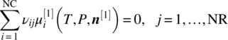
We consider a system comprising NC chemical compounds i = 1, …, NC that may be neutral or charged; the charge on compound i is denoted by qi. The compounds may take part in a number NR of chemical reactions j = 1, …, NR; the stoichiometric coefficient of compound i in reaction j is denoted by νij.
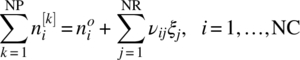
The compounds are distributed over a number NP of phases k = 1, …, NP. If the initial molar amount of compound i in the system is denoted by ![]() , then the amounts
, then the amounts ![]() of each compound i in each phase k at a given temperature T and pressure P are such that the total Gibbs free energy of the system is minimized. This leads to the following equilibrium conditions:
of each compound i in each phase k at a given temperature T and pressure P are such that the total Gibbs free energy of the system is minimized. This leads to the following equilibrium conditions:
- For each neutral compound i (qi = 0):
- For each pair of charged compounds
 :
:
- For each chemical reaction j:
- For each compound i:
- For each phase k:


where
![]() is the chemical potential of compound i in phase k; as indicated above, it is generally a function of temperature, pressure and the vector
is the chemical potential of compound i in phase k; as indicated above, it is generally a function of temperature, pressure and the vector ![]() of molar amounts of the compounds in phase k.
of molar amounts of the compounds in phase k.
ξj is the extent of reaction j = 1, …, NR.
We note that the chemical reaction equilibrium condition (19.3) is written arbitrarily in terms of the chemical potentials in phase 1. It can be shown that, because of the phase equilibrium conditions (19.1) and (19.2), this also holds for all other phases. Similarly, the electroneutrality condition (19.5) is omitted for phase 1 as it is implied by the material balance Eq. (19.4) and the fact that the overall system is neutral.
Conditions (19.1)–(19.5) constitute a system of NC × NP + NR equations that can be solved to determine the phase compositions ![]() and reaction extents ξj.
and reaction extents ξj.
The above mathematical formulation assumes that the number NP of phases in the system is known. In reality, this needs to be determined in an iterative manner that postulates a certain number of phases, solves the phase and reaction equilibrium problem, and then considers the stability of each individual phase at the equilibrium point. We will consider the phase stability problem in Section 19.2.5.
19.2.2 Fundamental Conditions for Solid–Liquid Equilibria
The conditions presented above are completely general and apply to any set of phases of any kind, with all compounds under consideration appearing in each and every phase. For solubility calculations in a pharmaceutical context, our interest is focused primarily on systems comprising only solid and liquid phases. Moreover, in most cases of interest, including those of simple APIs, API salts, hydrates and solvates, and co‐crystals, the solid phases have fixed composition, with a subset of the compounds in the system being present in fixed proportions. In fact, for the purposes of solubility calculations, it is convenient to think of these combinations as separate “compounds.” The latter may not exist in the liquid phases; instead, upon dissolution, they dissociate to their constituent compounds in a manner that can be described by an equilibrium chemical reaction. For example, in the case of a (2 : 1) co‐crystal A2.B between an API A and a coformer B, we have a dissociation reaction of the form
while a sodium salt of an acidic API may dissociate in an aqueous environment according to
We note that, although each solid phase comprises a single compound, the same compound may appear in multiple solid phases corresponding to different polymorphs. In general, at most one of these phases will appear in a nonzero amount at equilibrium, the others corresponding to metastable phases.1 Furthermore, in addition to the above solid–liquid dissociation reactions, the system may also involve reactions taking place entirely within the liquid phases.
In view of the above discussion, the general phase equilibrium conditions presented in Section 19.2.1 may be amended to take account of the specific features of the solubility calculation problem. The main modification required is to the phase equilibrium condition (19.1). Assuming, for simplicity, that phase 1 is always a liquid:
- For compounds i that exist both in solid and liquid phases (e.g. non‐dissociating or weakly dissociating APIs), Eq. (19.1) is modified to remove the composition dependence of the chemical potential in all solid phases
for any solid phase k comprising compound i. Note that Eq. (19.1) remains unchanged for other liquid phases k.
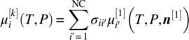
- For compounds i that exist exclusively in solid phases (e.g. API salts, hydrates or solvates, or co‐crystals), Eq. (19.1) is replaced by the equilibrium conditions for the corresponding dissociation reaction. These are a special case of Eq. (19.3), and can be written as
for any solid phase k comprising compound i. Here σii′ denotes the stoichiometry of composite compound i in terms of other compounds i′ in the system (i.e. one mole of compound i comprises
 moles of compound i′).
As an illustration, consider again the (2 : 1) co‐crystal and salt examples introduced earlier in this section in a system comprising one solid and one liquid phase. For these cases, Eq. (19.7) will take the form
and
respectively. Here ![]() denotes the entire vector of composition including the solvent(s), other ions (e.g. H+ and OH− for the salt example), etc.
denotes the entire vector of composition including the solvent(s), other ions (e.g. H+ and OH− for the salt example), etc.
On the other hand, for an API A that can also exist in the liquid phase, the relevant equation is (19.6), taking the simple form
19.2.3 Liquid‐Phase Chemical Potentials
The discussion in Sections 19.2.1 and 19.2.2 demonstrates that the only thermodynamic property required for solubility calculations is the chemical potential of each compound present in the system. In particular, there is no need for introducing concepts such as “reaction equilibrium constants” (or related quantities such as pKa) or “solubility products”. In this section, we consider the computation of liquid‐phase chemical potentials, while Section 19.2.4 focuses on solid‐phase chemical potentials.
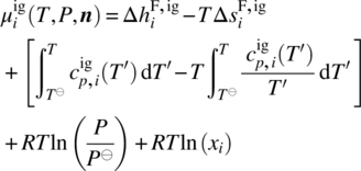
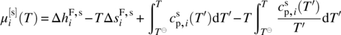
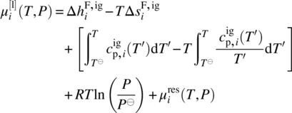
Since in general we need to be able to handle chemical transformations (e.g. dissociation of composite compounds from solid to liquid phases; liquid‐phase reactions), we need to adopt a reference datum of chemical elements at a reference temperature T⊖ and pressure P⊖. Thus, the chemical potential of a compound i in a liquid phase l can be computed by
where ![]() is the ideal gas chemical potential of compound i given by
is the ideal gas chemical potential of compound i given by
where
-
 and
and  are, respectively, the enthalpy and entropy of formation of compound i in the ideal gas standard state at temperature T⊖ and pressure P⊖.
 -
 is the ideal gas specific heat capacity of compound i.
 - xi is the molar fraction of compound i given by
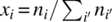 .
.
The quantity ![]() is the residual chemical potential of compound i, representing the difference between the real chemical potential and the ideal gas one under identical conditions of temperature, pressure, and composition.
is the residual chemical potential of compound i, representing the difference between the real chemical potential and the ideal gas one under identical conditions of temperature, pressure, and composition.
The liquid‐phase chemical potential may also be expressed in terms of reference states other than the ideal gas, such as the pure liquid state or a variety of infinite dilution states. In such cases, the residual term ![]() is replaced by a term based on the corresponding activity coefficient γi(T, P, n), which may be computed via a wide range of empirical and semiempirical models [7, 8]. However, as we shall see in Section 19.3, a significant development over the last decade has been the development of EoS that can accurately compute
is replaced by a term based on the corresponding activity coefficient γi(T, P, n), which may be computed via a wide range of empirical and semiempirical models [7, 8]. However, as we shall see in Section 19.3, a significant development over the last decade has been the development of EoS that can accurately compute ![]() over wide ranges of conditions for general liquid mixtures involving different types of molecules (e.g. neutral compounds, ions, polymers) and complex intermolecular interactions including hydrogen bonding or other forms of association and electrostatic (coulombic) forces. Moreover, the group contribution basis of these EoS implies that they can be applied to systems for which little experimental data are available.
over wide ranges of conditions for general liquid mixtures involving different types of molecules (e.g. neutral compounds, ions, polymers) and complex intermolecular interactions including hydrogen bonding or other forms of association and electrostatic (coulombic) forces. Moreover, the group contribution basis of these EoS implies that they can be applied to systems for which little experimental data are available.
In view of the above, our approach to computing solubilities is based on Eqs. (19.8) and (19.9). It is worth noting that, contrary to what is sometimes stated in the literature, these equations are applicable to any type of compound. In cases where experimentally derived values for the enthalpy and entropy of formation are available for reference states other than the ideal gas, they can easily be converted to the quantities ![]() and
and ![]() required by Eq. (19.9) using the EoS itself. For example, the enthalpy
required by Eq. (19.9) using the EoS itself. For example, the enthalpy ![]() and entropy of formation
and entropy of formation ![]() of a pure liquid at temperature T⊖ and pressure P⊖ are related to the corresponding ideal gas quantities via
of a pure liquid at temperature T⊖ and pressure P⊖ are related to the corresponding ideal gas quantities via
where the residual enthalpy ![]() and entropy
and entropy ![]() of the pure liquid can be obtained from the corresponding
of the pure liquid can be obtained from the corresponding ![]() computed by the EoS via the standard thermodynamic relations:
computed by the EoS via the standard thermodynamic relations:
Similar relations can be derived for enthalpies and entropies of formation in infinite dilution reference states and are presented in Appendix 19.A.
Figure 19.1 summarizes the different approaches to computing liquid‐phase chemical potentials in the form of thermodynamic paths from chemical elements at standard conditions (T⊖, P⊖) to the mixture under the conditions (T, P, n) of interest. Different paths make use of formation properties corresponding to different reference states. All these quantities can be interconverted to each other via the use of an EoS that can accurately compute residual properties of pure compounds. This allows the use of whatever experimentally determined values of formation properties happen to be available, even if these are with respect to different reference states for different compounds in the system under consideration.
FIGURE 19.1 Summary of the various possible thermodynamic paths for the computation of chemical potential of compound i in liquid phases  using formation properties at different standard states. The thermodynamic integration path depends on whether an equation of state (EoS) or activity coefficient model (ACM) is used to model the mixture nonidealities.
All calculations reported in this chapter make use of the thermodynamic path going through the ideal gas reference state as shown by the solid arrows in Figure 19.1. For completeness, this diagram also shows paths based on activity coefficient models as dashed arrows.
19.2.4 Solid‐Phase Chemical Potentials
We now turn our attention to the computation of solid‐state chemical potentials of the kind that appear in the phase equilibrium conditions (19.6) and (19.7).
Below we consider two alternative approaches that differ in their requirements for solid‐state properties. In particular, the approach described in Section 19.2.4.1 makes use of enthalpy and entropy of formation, while that described in Section 19.2.4.2 relies on properties related to the melting of the solid phase.
19.2.4.1 Solid‐Phase Potentials in Terms of Formation Properties
Although, in principle, Eq. (19.8) holds for solid phases too, there is currently no generally applicable way of computing the residual term ![]() . In particular, both EoS and activity coefficient models are restricted to phases exhibiting liquid‐like structures only, and cannot describe the behavior of phases where the underlying microscopic structure follows a well‐defined geometric pattern such as crystalline solid phases.2
. In particular, both EoS and activity coefficient models are restricted to phases exhibiting liquid‐like structures only, and cannot describe the behavior of phases where the underlying microscopic structure follows a well‐defined geometric pattern such as crystalline solid phases.2
In view of the above, we express the chemical potential of a compound i in a solid phase corresponding to a particular crystal structure as
where
-
 and
and  are, respectively, the enthalpy and entropy of formation of the solid phase of the same crystal structure at standard temperature T⊖ and pressure P⊖.
 -
 is the specific heat capacity of the solid at temperature T and pressure P⊖.
The above equation omits the pressure dependence of ![]() as this is typically very small at the pressures of interest to pharmaceutical applications.
as this is typically very small at the pressures of interest to pharmaceutical applications.
19.2.4.2 Solid‐Phase Potentials in Terms of Melting Properties
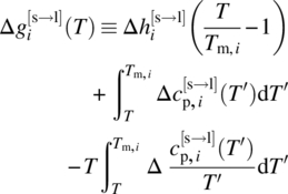
The melting properties approach takes advantage of the fact that at the melting point temperature Tm,i of pure compound i, its liquid‐ and solid‐phase chemical potentials (i.e. free energy) are equal. Neglecting pressure effects and integrating along the thermodynamic path [3]
we obtain the following expression for the solid chemical potential:
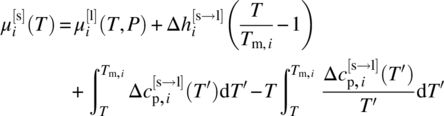
where
-
 is the enthalpy of melting at Tm,i.
 -
 is the difference between liquid‐ and solid‐specific heat capacities.
Since T < Tm,i, the chemical potential ![]() corresponds to a metastable (subcooled) liquid phase but can nevertheless be computed from an EoS.
corresponds to a metastable (subcooled) liquid phase but can nevertheless be computed from an EoS.
This approach is usually applied to APIs that are stable up to their melting points. In principle, it can be extended to co‐crystals and salts which also have a well‐defined, experimentally measurable melting point. In that case, the liquid‐phase properties (chemical potential and specific heat capacity) used in the expression in the right‐hand side of Eq. (19.13) need to be replaced by those of a liquid‐phase mixture with the fixed composition as dictated by the stoichiometric makeup of compound i (cf. Section 19.2.2).
19.2.5 Determination of Solid Phases Present in the System
The phase equilibrium conditions underpinning solubility calculations (cf. Section 19.2.2) assume that both the number NP of phases that are present in the system and their nature (liquid mixtures; solids of various types) are known. In reality, given the molar amounts ![]() of the compounds i = 1, …, NC under consideration, we need to establish the complete set of phases that are present at the temperature T and pressure P of interest. One approach for achieving this aim is to start with a single liquid phase comprising all of the specified amounts and then test its stability with respect to all solid phases that may potentially form given the set of compounds under consideration.3 For the general systems considered here, any nonzero amounts
of the compounds i = 1, …, NC under consideration, we need to establish the complete set of phases that are present at the temperature T and pressure P of interest. One approach for achieving this aim is to start with a single liquid phase comprising all of the specified amounts and then test its stability with respect to all solid phases that may potentially form given the set of compounds under consideration.3 For the general systems considered here, any nonzero amounts ![]() of compounds i that exist only in solid phases (e.g. co‐crystals) can be converted to the equivalent amounts σii′ of the compounds i′ formed by their dissociation (cf. Eq. 19.7). The resulting liquid phase can then be equilibrated with respect to any chemical reactions taking place in it.
of compounds i that exist only in solid phases (e.g. co‐crystals) can be converted to the equivalent amounts σii′ of the compounds i′ formed by their dissociation (cf. Eq. 19.7). The resulting liquid phase can then be equilibrated with respect to any chemical reactions taking place in it.
A widely applied stability criterion is that based on the Gibbs surface tangent plane [7]. Given a fluid phase of composition n, it tests whether the formation of an infinitesimally small amount of a new “trial” phase would result in an overall reduction of the Gibbs free energy. If no such trial phase can be found, the original fluid phase is deemed to be stable. Mathematically, this is equivalent to requiring that the quantity
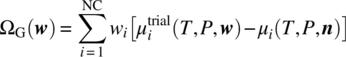
is nonnegative for any trial composition w.
The application of the above criterion in cases where the trial phase is a fluid is a complex problem that has been studied extensively in the literature. The main challenge is to ensure that ΩG(w) ≥ 0 for all possible nonzero w, something that can be formally guaranteed only via the use of techniques that systematically search over the entire range of trial compositions, e.g. via the use of global optimization algorithms [10–13].
However, testing stability of a liquid phase with respect to solid trial phases comprising a single compound is a significantly simpler problem. Because such phases comprise a single compound i, criterion (19.14) simplifies
- for compounds i that exist in both the solid and the liquid phases:(19.15a)

- for compounds i that dissociate into other compounds in the liquid phase (cf. Eq. 19.7):(19.15b)
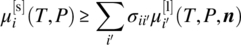
Given a liquid phase of composition n, the above stability criteria can easily be checked for each and every solid phase s under consideration using the values of the liquid‐ and solid‐phase chemical potentials (cf. Sections 19.2.3 and 19.2.4, respectively). If the criterion is found to be violated for any phase s, then that phase may be present in the system and therefore must be added to the set of phases included in the formulation of the phase equilibrium conditions presented in Section 19.2.2. The solution of these equations will then yield a new liquid‐phase composition n, which again can be tested for stability against potential existence of more solid phases. The above procedure is therefore repeated until a stable liquid phase is obtained.
It should be noted that for a given liquid‐phase composition, more than one trial solid phase may be found to violate the stability criterion (19.15). Our approach in such cases is to tentatively add each such solid phase s separately to the system, perform the associated solubility calculation, and then use the resulting equilibrium compositions to compute the total Gibbs free energy of the system:
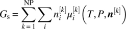
The trial solid phase s that results in the lowest free energy Gs is selected to be added to the system, and the corresponding liquid‐phase composition is subjected to further stability tests as described above.
19.3 THE SAFT‐γ MIE GROUP CONTRIBUTION EoS
In Section 19.2 we showed that the general problem of computing the solubility (and stability) for any type of pharmaceutical system relies on solving for a set of equations that are expressed entirely in terms of liquid‐ and solid‐phase chemical potential. The complexity of the solubility calculation is mainly due to the composition dependence of the liquid‐phase chemical potentials, whereas the solid phase is always a function of temperature only.
Therefore a prerequisite for the successful prediction of solubility is the choice of a suitable approach to compute the liquid‐phase chemical potentials of complex multifunctional molecular structures, which are ubiquitous in pharmaceutical applications. The general framework of the statistical associating fluid theory (SAFT) [14, 15] has been shown to be particularly promising in this context, having been successfully applied to a wide range of systems; see the reviews in Refs. [16–18] for a more extensive discussion. SAFT takes explicit account of intermolecular forces, incorporating the description of nonidealities due to asymmetry in molecular shape and anisotropic interactions. The fact that this theoretical framework is based on a physically sound representation of the APIs makes it one of the most promising approaches to date for the solubility prediction in solvent mixtures.
In this contribution, all the calculations are performed using the SAFT‐γ Mie group contribution approach [19, 20], a variant of the general SAFT framework based on a generalized Lennard‐Jones (or so‐called Mie) potential. As in other group contribution approaches, molecules are described in terms of the functional (chemical) groups they comprise. The functional groups are assumed to behave independently of the molecular structure on which they are found. An example of the decomposition of a molecular structure into the functional groups is given for the particular case of ibuprofen in Figure 19.2.

FIGURE 19.2 Decomposition of ibuprofen into functional groups (3 × CH3, 1 × CH, 1 × aCCH2, 4 × aCH, 1 × aCCH, 1 × COOH).
19.3.1 Intermolecular Potential Model
Within the SAFT‐γ Mie EoS, each functional group k is characterized by a shape factor parameter Sk, describing the group non‐sphericity as well as a set of parameters that relate to various group‐group interactions, as described below.
Repulsive and dispersive interactions are modeled via the Mie potential and are considered for all group pairs. On the other hand, hydrogen bonding interactions are included only where necessary (i.e. for groups that exhibit association interactions) and are modeled using short‐ranged square‐well sites. It is also possible to formally take into account the presence of permanent charges on functional groups. This allows for the rigorous (and explicit) modeling of the speciation of APIs in aqueous mixtures as will be shown in Section 19.5. This does not require any additional parameters besides the charge itself (positive or negative), which is always known a priori, thus making the extension to charged systems straightforward.
The parameters that describe the Mie intermolecular potential are the diameter σ, the repulsive and attractive exponents λrep and λatt, respectively, and the potential depth ɛ. The association interactions between pair of sites (denoted, for example, as a and b) are, if present, described by two additional parameters, namely, the energy of interaction, ![]() , and the volume available for bonding,
, and the volume available for bonding, ![]() . Note that no additional parameters are required for describing the formation of the molecular chains; this contribution is inferred by the knowledge of the distinct types of functional groups that comprise each molecule and their multiplicity on the molecular chains. Finally, the type and number of different association sites on a given group need to be defined a priori based on chemical understanding of hydrogen bonding donors and acceptors.
. Note that no additional parameters are required for describing the formation of the molecular chains; this contribution is inferred by the knowledge of the distinct types of functional groups that comprise each molecule and their multiplicity on the molecular chains. Finally, the type and number of different association sites on a given group need to be defined a priori based on chemical understanding of hydrogen bonding donors and acceptors.
The interaction parameters described above relate to all pair interactions. A schematic representation of the physical meaning of each parameter is given in Figure 19.3. In practice, when developing the group pair interaction parameters, we commonly separate the treatment of the groups that are of the same type (self‐interactions) and the interactions between groups of different types (unlike or cross‐interactions). The self‐interaction parameters are almost always obtained by regression to experimental data, whereas the parameters that describe unlike interaction can be approximated by combining rules. Overall, the application of the SAFT‐γ Mie approach for pharmaceutical system relies on the development of databases of group interaction parameters for relevant chemical groups typically found in APIs. Section 19.3.2 explains the procedure for developing such database based on experimental data.
FIGURE 19.3 Schematic representation of the SAFT‐γ Mie parameters needed to describe the group self‐ and cross‐interactions. The choice of the association scheme for the COOH and H2O groups is discussed in detail in Ref. [21].
Source: Reproduced with permission of Elsevier.
19.3.2 Estimation of Group Parameters from Experimental Data
As we have seen in Section 19.3.1, most of the parameters in the SAFT‐γ Mie EoS relate to interactions between functional groups. In practice, one can make use of available experimental data on simple systems to estimate these in a sequential manner.
When using a group contribution EoS such as SAFT‐γ Mie, a wide range of different data types can be used, including not only data on the thermodynamic properties and phase behavior of binary and/or multicomponent systems but also pure component data (single phase and equilibrium). This is a significant benefit over activity coefficient models, since only EoS approaches can be applied to the description of pure components and, hence, benefit from the availability of readily available pure component data in the development of group parameters.
In order to obtain reliable parameter estimates, a commonly used strategy is to include various types of experimental data in the regression procedure, including, for instance, densities, vapor pressure, and caloric data (heat capacity and/or vaporization enthalpy). The key aspect of the SAFT‐γ Mie group contribution methodology is that experimental data on any molecule containing the group of interest can be used in the regression procedure. In principle, a database of group parameters relevant to pharmaceutical applications can be developed without the use of API‐specific data.
The details on the exact sequence of development of all the functional group interactions used in the application section (Section 19.5) are beyond the scope of this chapter, but it is worth considering the simple example of CH3, CH2, and OH groups to illustrate the general workflow. First the methyl and methylene groups can be obtained by regression to experimental data for a series of (pure) n‐alkanes, from ethane to n‐decane. Having determined the parameters for the CH3 and CH2 groups, the OH group can then be obtained using primary alcohol data. Note that the usage of pure component data allows the determination of not only the self‐interactions but also the cross‐interactions between each group pair. A similar sequence can then be used to determine any other group, by selecting either pure component or mixture data.
Finally, it is worth noting that the SAFT‐γ Mie EoS can be used in a “molecular” mode, with an entire compound being represented as a single functional group. This is typically the case for the first member of each chemical family – e.g. methane for the n‐alkanes; methanol for the alcohols; etc. – but can also be employed in the study of more complex molecules. Note that in such cases compound‐specific experimental data are required for the development of the (single) group parameters.
19.4 SYSTEM CHARACTERIZATION FOR SOLUBILITY CALCULATIONS
As described in Section 19.2.2, the computation of solid–liquid equilibria requires accurate values of the chemical potential of the individual compounds in the liquid and solid phases using the approaches presented in Sections 19.2.3 and 19.2.4, respectively, and, in particular, Eqs. (19.8), (19.9), (19.12), and (19.13).
This section focuses on the parameters that are required by these equations, and the way in which they can be obtained from experimental data. Section 19.4.1 provides a summary and categorization of the relevant parameters.
Because of the fundamental thermodynamic approach adopted in this chapter, these parameters are not specific to solubility calculations; in fact, most of them can be obtained or estimated without access to experimental solubility data. However, even limited availability of such data for the specific API of interest can substantially reduce the effort required for accurate solubility prediction. Interestingly, this may be true even if the available data pertain to completely different solvents or solvent mixtures to the ones involved in the system of interest. This is possible because of the use of predictive EoS such as the SAFT‐γ Mie (cf. Section 19.3).
More specifically, Section 19.4.2 considers the use of experimental solubility data for the characterization of the solid state of solid‐forming compounds that also exist in the liquid phase. Section 19.4.3 covers the same topic for compounds such as API salts, solvates, hydrates, and co‐crystals that only exist in the solid phase, dissociating into other compounds in the liquid phase. Finally, Section 19.4.4 considers the characterization of liquid‐phase chemical reactions using data from any system that contains a liquid phase in which these reactions occur. The use and power of all of these techniques will be demonstrated extensively in the examples considered in Section 19.5.
19.4.1 Parameters Involved in Solubility Calculations
Equations (19.8), (19.9), (19.12), and (19.13) involve a number of parameters:
- Pure compound parameters
- Enthalpies and entropies of formation in the ideal gas reference state at standard temperature T⊖ and pressure P⊖.
- Parameters describing the temperature dependence of specific heat capacities in the ideal gas state.
- Either
-
- Enthalpies and entropies of formation of crystalline phases at standard temperature T⊖ and pressure P⊖.
- Parameters describing the temperature dependence of solid‐phase specific heat capacities.
- or
-
- Melting point temperature and enthalpy of melting at that temperature.
- Parameters describing the temperature dependence of the difference between liquid‐ and solid‐phase specific heat capacities.
- EoS parameters used for the computation of liquid‐phase chemical potentials and related quantities, including:
- Residual chemical potentials used in Eq. (19.8).
- Pure compound potential used in Eq. (19.13).
- (Optionally) the terms required for obtaining the ideal gas formation properties from values of formation properties in other reference states as shown, for example, in Eqs. (19.10) and (19.11).
Some of these parameters can be estimated using group contribution methods, such as the Joback and Reid [22] method for ideal gas specific heat capacities. Others may be determined experimentally either via direct measurement (e.g. melting parameters using DSC techniques) or indirect estimation from experimental data (e.g. formation enthalpies and entropies). As already mentioned in Section 19.3, in the case of the SAFT‐γ Mie EoS parameters for the various functional groups, these experimental data could relate to fluid‐phase measurements (e.g. vapor–liquid or liquid–liquid equilibria) obtained from systems that do not actually involve any of the compounds occurring in the system of interest.
19.4.2 Solid‐Forming Compounds That Also Exist in the Liquid Phase
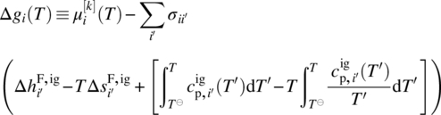
We start by revisiting the equilibrium condition (19.6) for compounds that exist in both the liquid and solid phases. Using Eqs. (19.8) and (19.9), ignoring the pressure dependence of the solid‐phase potential and applying some minor rearrangement, we obtain an expression of the form

where we have introduced a new quantity ∆gi defined as

and have retained the phase labeling conventions of the original Eq. (19.6), i.e. k denotes the solid phase formed by compound i and phase “1” is a liquid phase.
We note that the definition (19.18) implies that ∆gi(T) is purely a characteristic of the solid‐forming compound i and does not depend on any other compound in the system, and that it is solely a function of temperature. Therefore the value of ∆gi(T) for a given solid API i at a given temperature T will always be the same, irrespective of the system in which this API occurs. Moreover, turning to Eq. (19.17), we can see that we can compute this ∆gi(T) from any available experimental solubility data for this API by using the measured liquid‐phase composition to replace the quantities ![]() and
and ![]() appearing in the right‐hand side – provided, of course, we have an EoS that can compute the residual term
appearing in the right‐hand side – provided, of course, we have an EoS that can compute the residual term ![]() .
.
It is worth noting that the original equilibrium condition (19.6) between solid phase k and liquid phase 1 is valid irrespective of the existence of other solid and/or liquid phases. Therefore, this type of calculation is correct even if the experimental data were derived in systems with multiple solid and/or liquid phases. It is sufficient to have the measured composition of one of the liquid phases.
As an illustration, Figure 19.4 shows the function ∆gi(T) for ibuprofen. The values shown are computed from the right‐hand side of Eq. (19.17) using published experimental solubility data [23–26] from a range of solvents over a range of temperatures, with the ![]() term being computed via the SAFT‐γ Mie EoS. It is clear that all the points define a single function, irrespective of the solvent being considered and the actual solubility values. Moreover, at least in this case, this function can be well approximated by a straight line empirically determined to be of the form ∆gibuprofen(T) = 238.78T − 117 460 (∆gibuprofen in J/mol, T in K).
term being computed via the SAFT‐γ Mie EoS. It is clear that all the points define a single function, irrespective of the solvent being considered and the actual solubility values. Moreover, at least in this case, this function can be well approximated by a straight line empirically determined to be of the form ∆gibuprofen(T) = 238.78T − 117 460 (∆gibuprofen in J/mol, T in K).
FIGURE 19.4 Calculation of empirical model for Δgi(T) for ibuprofen.
Once the function ∆gi(T) for a given API i has been determined, it can be used directly for the computation of its solubility within any solvent or solvent mixture simply by using Eq. (19.17) to replace the original condition (19.6) in the solubility calculations. Importantly, the values of the various pure compound parameters appearing on the right‐hand side of Eq. (19.18) are not necessary. Effectively, the use of an advanced EoS allows transferability of solubility information from one system (or systems) to another.
As mentioned in Section 19.2.4.2, an alternative to the use of solid‐phase chemical potentials based on formation energies (Eq. 19.12) is to employ an expression based on melting properties as indicated by Eq. (19.13). The latter requires knowledge of the pure liquid chemical potential ![]() , which can itself be calculated using Eqs. (19.8) and (19.9):
, which can itself be calculated using Eqs. (19.8) and (19.9):
where the last term on the right‐hand side is the residual chemical potential for the pure liquid that can be calculated using the EoS. It will be noted that the above does not include the +RT ln(xi) term that appears on the right‐hand side of Eq. (19.9) as xi = 1 for the case of pure liquid.
The expression for ![]() given by Eq. (19.19) can then be substituted in Eq. (19.13) to yield a complete expression for the solid‐phase chemical potential
given by Eq. (19.19) can then be substituted in Eq. (19.13) to yield a complete expression for the solid‐phase chemical potential ![]() . The latter may then be used on the left‐hand side of equilibrium condition (19.6), with Eqs. (19.8) and (19.9) being used to compute the liquid‐phase chemical potential
. The latter may then be used on the left‐hand side of equilibrium condition (19.6), with Eqs. (19.8) and (19.9) being used to compute the liquid‐phase chemical potential ![]() on the right‐hand side. At this point, all terms arising from the right‐hand side of Eq. (19.19) except the last one will appear identically on both sides and will cancel out, resulting in an equation of the form
on the right‐hand side. At this point, all terms arising from the right‐hand side of Eq. (19.19) except the last one will appear identically on both sides and will cancel out, resulting in an equation of the form
where the quantity ![]() is defined as
is defined as
Analogously to the quantity ∆gi(T) defined by Eq. (19.18), ![]() is purely a characteristic of compound i and is solely a function of temperature. It can, therefore, also be described by an empirical relationship derived by fitting values obtained by computing the right‐hand side of Eq. (19.20) at available experimental data points. On the other hand, if the melting properties
is purely a characteristic of compound i and is solely a function of temperature. It can, therefore, also be described by an empirical relationship derived by fitting values obtained by computing the right‐hand side of Eq. (19.20) at available experimental data points. On the other hand, if the melting properties ![]() and
and ![]() of compound i are known, then they can be used directly for the computation of
of compound i are known, then they can be used directly for the computation of ![]() using Eq. (19.21) without the need to resort to experimental solubility data. In either case, there is no need to know the ideal gas properties
using Eq. (19.21) without the need to resort to experimental solubility data. In either case, there is no need to know the ideal gas properties ![]() , and
, and ![]() .
.
19.4.3 Solid‐Forming Compounds That Exist Only in the Solid Phase
As already mentioned in Section 19.2.2, API salts, solvates, hydrates, and co‐crystals are assumed to exist only in the solid phase, dissociating fully upon entering the liquid phase. In such cases, the relevant equilibrium condition is Eq. (19.7). By following an approach similar to that used for the simpler case considered in Section 19.4.2 above, we can derive the equation
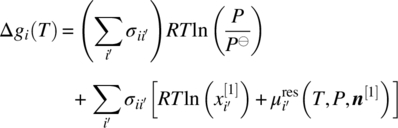
where the quantity ∆gi is now defined as
As in the previous case, Eq. (19.23) shows that ∆gi(T) is a characteristic of the compound i under consideration (e.g. a particular co‐crystal) and is solely a function of temperature. Inserting any available experimental solubility data for this compound on the right‐hand side of Eq. (19.22) allows us to compute the corresponding ∆gi(T) and fit an empirical function of temperature to it. The latter can then be used in conjunction with Eq. (19.22) instead of the original condition (19.7) to compute solubilities of compound i in other systems of interest. Once again, we do not actually need to know any of the pure compound quantities appearing on the right‐hand side of Eq. (19.23).
19.4.4 Characterization of Liquid‐Phase Chemical Reactions
Liquid‐phase chemical reactions are described by the chemical equilibrium condition (19.3). Following an approach similar to that presented in Sections 19.4.2 and 19.4.3, the latter can be reformulated to an equation of the form
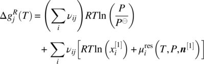
where the quantity ![]() is now defined as
is now defined as

From Eq. (19.25), we note that the free energy quantity ![]() is a characteristic of the particular chemical reaction j and depends only on temperature. As before, we can follow a two‐step procedure:
is a characteristic of the particular chemical reaction j and depends only on temperature. As before, we can follow a two‐step procedure:
- Determine the values of this quantity at different temperatures by computing the expression on the right‐hand side of Eq. (19.24) using experimentally measured liquid‐phase compositions for any system4 in which this reaction occurs.
- Use the values computed above to fit an empirical expression (e.g. a linear or quadratic relation) to describe the temperature variation of
 .
.
Once we have the empirical expression ![]() , we can use it for characterizing reaction j in any system of interest where it may occur by replacing the original equilibrium condition (19.3) by Eq. (19.24).
, we can use it for characterizing reaction j in any system of interest where it may occur by replacing the original equilibrium condition (19.3) by Eq. (19.24).
It is worth noting that it is not always possible to measure directly the complete liquid‐phase composition. For instance,5 in aqueous ionic systems what is typically measured is the pH (i.e. the activity of the H+ ion) and the API total molar fraction, which comprises contributions from both the undissociated API and its ion(s). In such cases, step 1 of the above procedure needs to be amended as it is no longer possible to explicitly compute ![]() at the experimental temperature T simply by evaluating the right‐hand side of Eq. (19.24). Instead, the latter needs to be considered simultaneously with the material balance Eq. (19.4) to determine the value of
at the experimental temperature T simply by evaluating the right‐hand side of Eq. (19.24). Instead, the latter needs to be considered simultaneously with the material balance Eq. (19.4) to determine the value of ![]() that leads to the best fit of the available measurements.
that leads to the best fit of the available measurements.
19.5 ILLUSTRATIVE EXAMPLES
This section presents a number of examples illustrating the key aspects of the general framework for solid–liquid equilibria presented in this chapter and demonstrating its applicability to systems of relevance to pharmaceutical applications.
Section 19.5.1 provides a brief overview of a computer implementation of this framework. Sections 19.5.2–19.5.7 present solid–liquid equilibrium calculations for six different systems involving:
- One or more different types of solid phases (unionizable or weakly acidic APIs, API salts, hydrates, co‐crystals, and polymers).
- Pure organic solvents and their mixtures.
- Aqueous systems with pH‐modifying agents.
Particular emphasis is paid to the characterization of liquid‐ and solid‐phase behavior from practically available experimental data.
Finally, Section 19.6 attempts to draw some more general conclusions from these examples.
19.5.1 The gSAFT Physical Properties Code
All calculations presented in this section were performed using gSAFT [27], a physical properties code developed by Process Systems Enterprise Ltd. for use within its gPROMS® [28] process modeling tool.
Designed to support pharmaceutical applications in the context of drug substance and drug product manufacturing and also oral absorption, gSAFT incorporates several elements of relevance to the topic of this chapter:
- An algorithm for the reliable computation of equilibria in multiple vapor–liquid–solid phases in the presence of chemical reactions, based on the general equilibrium conditions presented in Section 19.2.1 and including a comprehensive phase stability analysis (cf. Section 19.2.5).
- A robust implementation of the SAFT‐γ Mie EoS (cf. Section 19.3) that can be applied efficiently to mixtures with large numbers of neutral and/or charged compounds in the presence of association and/or coulombic interactions.
- A database of SAFT‐γ Mie parameters for functional groups commonly occurring in organic and aqueous systems, including a range of (mainly inorganic) ions.
- A tool for the reliable6 estimation of SAFT‐γ Mie parameters from multiple data sets derived from a range of standardized experiments such as pure compound vapor pressures and saturated liquid densities, vapor–liquid or liquid–liquid phase equilibria for binary mixtures, solubility measurements in single solvents or solvent mixtures, titration curves, etc.
- A tool for the derivation of empirical models for the temperature dependence of quantities:
- ∆gi(T) and
 from experimental solubility measurements (cf. Sections 19.4.2 and 19.4.3).
 -
 from experimental liquid‐phase composition measurements (cf. Section 19.4.4).
- ∆gi(T) and
In addition to SAFT‐γ Mie, gSAFT also incorporates implementations of the SAFT‐VR SW [29, 30] and PC‐SAFT [31, 32] EoS and associated databanks. In principle, these EoS can also be used to perform solid–liquid equilibrium calculations within the framework described in this chapter (see, for example, [33–36]). However, they require parameters to be estimated specifically for each individual API, typically using experimental solubility data. This is in contrast to SAFT‐γ Mie EoS, which, by virtue of its functional group basis, is capable of making use of experimental information from systems involving different compounds and/or phases. This advantage of SAFT‐γ Mie EoS is particularly pronounced in systems involving complex molecules (such as pharmaceutical APIs) for which relatively little experimental data may be available.
19.5.2 Example 1: Solubility of Fenofibrate in Alcohols
The molecular structure of fenofibrate and its decomposition into functional groups is presented in Figure 19.5. The parameters for all the functional groups are already available within the gSAFT databank, having been estimated entirely from published experimental data derived from fluid‐phase experiments; no solubility data of any kind were used for this purpose.

FIGURE 19.5 Molecular structure of fenofibrate (propan‐2‐yl 2‐{4‐[(4‐chlorophenyl)carbonyl]phenoxy}‐2‐methylpropanoate) and its decomposition into functional groups in SAFT‐γ Mie.
The solid‐phase chemical potential is computed using the melting point approach described in Section 19.2.4.2, with the experimentally measured values of melting temperature and melting enthalpy reported in [37]. The specific heat capacity difference ![]() was set to zero.
was set to zero.
The approach described in this chapter is now used to predict the solubility of fenofibrate in ethanol and 1‐propanol.7 A comparison between the predicted values and experimental data reported in the literature is shown in Figure 19.6. The solubility is presented as the liquid‐phase molar fraction of fenofibrate, with a logarithmic scale being employed to allow a clearer inspection of the low solubility values. It can be seen that the predictions are in good agreement with the experimental data, the slight deviations being attributed to the fact that some of the unlike interactions between functional groups of the solute and the solvents are approximated by means of combining rules, and have not been regressed using experimental data.

FIGURE 19.6 Mole fraction solubility of fenofibrate in (a) ethanol and (b) 1‐propanol. The solid form of fenofibrate was described using melting properties (Tm = 352.05 K, Δh[s → l](Tm) = 33.53 kJ/mol [37]). The circles represent experimental data [37, 38] and the lines are pure predictions by gSAFT; no experimental solubility data of any kind were used in fitting model parameters.
Source: Adapted from Watterson et al. [37] and Sun et al. [38].
In order to assess further the predictive capability of SAFT‐γ Mie, we present in Figure 19.7 the computed solubilities in a binary mixture of water + ethanol. In general the computation of solubilities of APIs in a mixture of solvents is straightforward in gSAFT, the accuracy of the prediction depending on whether the majority of the group cross‐interactions available in the gSAFT database have been regressed using experimental data, instead of being approximated by combining rules.

FIGURE 19.7 Mole fraction solubility of fenofibrate in a binary mixture of water + ethanol. The circles and squares represent experimental data [38] and the lines are pure predictions by gSAFT.
Source: Reproduced with permission of American Chemical Society.
19.5.3 Example 2: Solubility of Ibuprofen in PEG Polymers
This example considers the solubility of ibuprofen in polyethylene glycol polymer of given molecular weight (MW = 10 000 g/mol), an application of relevance to the solubilization of APIs with poor aqueous solubility via the preparation of solid dispersions. The molecular structure of ibuprofen and its decomposition into functional groups in gSAFT are presented in Figure 19.8.
FIGURE 19.8 Molecular structure of ibuprofen (2‐(4‐(2‐methylpropyl)phenyl)propanoic acid) and its decomposition into functional groups in SAFT‐γ Mie.
The functional group decomposition of the PEG polymer is shown in Figure 19.9. The group contribution basis of SAFT‐γ Mie provides a natural mechanism for modeling complex polymers of arbitrary molecular weight. For example, PEG of molecular weight 10 000 g/mol is described as 2 hydroxyl groups combined with 454 methylene groups and 226 ether groups.
FIGURE 19.9 Molecular structure of PEG and its decomposition into functional groups in SAFT‐γ Mie.
The melting point approach was used for the characterization of the solid phases of both ibuprofen and PEG, with the corresponding melting temperatures and enthalpies shown in Table 19.1. The specific heat capacity differences ![]() were set to zero.
were set to zero.
TABLE 19.1 Solid‐Phase Characterization for Ibuprofen and PEG 10000 System
| Compound | Solid‐Phase Characterization |
| Ibuprofen | Tm = 347.15 K [23] Δh[s → l](Tm) = 25.50 kJ/mol [23] |
| PEG 10000 | Tm = 331.05 K [39] Δh[s → l](Tm) = 3360.0 kJ/mol [39] |
| IB5.PEG | Δg(T) = − 381.344 − 0.806 95 T (in kJ/mol; fitted) |
Experimental data for this particular system [39] suggest the potential appearance of a co‐crystal with a 5 : 1 ibuprofen‐to‐PEG ratio, reflecting the experimental composition at which the solid‐liquid equilibrium temperature exhibits a maximum. Within our general framework for solid–liquid equilibria, the co‐crystal is considered as a compound that appears only in a solid phase, dissociating to its constituents in the liquid phase:
Moreover, in view of the lack of the necessary solid‐phase data, we characterize this compound using the approach described in Section 19.4.3 to derive an empirical representation for the function Δgi(T). In this case, we assume that the latter has a simple linear form obtained by drawing a straight line through two experimental solubility data points (shown by black circles in Figure 19.10). The resulting empirical model is also shown in Table 19.1.
FIGURE 19.10 Solid–liquid phase diagram of ibuprofen + PEG 10000 g/mol assuming the formation of a co‐crystal IB5.PEG. Circles represent experimental data [39] and lines are gSAFT predictions. The latter made use of a linear empirical model of the co‐crystal free energy function Δgi(T) (cf. Eq. 19.23) derived from only two experimental solubility data points shown as filled black circles.
Based on this information, we can now trace the entire solid–liquid phase diagram for this system over a range of temperatures T and ibuprofen mass fractions w. This is shown in Figure 19.10, where the lines represent calculations obtained using SAFT‐γ Mie and the symbols the experimental solubility points. It can be seen that starting off with a liquid solution at a given temperature, a range of different solid forms can be obtained upon cooling depending on the initial composition.
19.5.4 Example 3: Solubility of Ketoprofen in PEG Polymers
This example examines the solubility of ketoprofen in PEG of molecular weight 6000 g/mol. The molecular structure and functional group decomposition of ketoprofen are shown in Figure 19.11.
FIGURE 19.11 Molecular structure of ketoprofen (2‐(3‐benzoylphenyl)propanoic acid) and its decomposition into functional groups in SAFT‐γ Mie.
Experimental data [40] suggest the potential formation of a co‐crystal with a 10 : 1 ratio of ketoprofen to PEG. As in the previous example, the co‐crystal is considered as a compound that appears only in a solid phase, dissociating to its constituents in the liquid phase:
The approach used for the characterization of the solid‐phase behavior of ketoprofen, PEG 6000, and the KT10.PEG co‐crystal is identical to that adopted for the ibuprofen/PEG 10000 system presented in the previous Section 19.5.3. The parameters used for the solid–liquid equilibrium calculations are summarized in Table 19.2.
TABLE 19.2 Solid‐Phase Characterization for Ketoprofen and PEG 6000 System
| Compound | Solid‐Phase Characterization |
| Ketoprofen | Tm = 368.00 K [40] Δh[s → l](Tm) = 37.30 kJ/mol [40] |
| PEG 6000 | Tm = 336.78 K [41] Δh[s → l](Tm) = 1182.0 kJ/mol [41] |
| KT10.PEG | Δg(T) = − 305.767 − 0.425399 T (in kJ/mol; fitted) |
A comparison between the predictions obtained using the SAFT‐γ Mie approach and the experimental solubility data is presented in Figure 19.12. The latter illustrates both the complexity of the phase diagram and the accuracy of the proposed approach to the computation of solid–liquid equilibria.
FIGURE 19.12 Solid–liquid phase diagram of ketoprofen + PEG 6000 g/mol assuming the formation of a co‐crystal KT10.PEG. Circles represent experimental data [41] and lines are gSAFT predictions. The latter made use of a linear empirical model of the co‐crystal free energy function Δgi(T) (cf. Eq. 19.23) derived from the two experimental solubility data points shown as filled black circles.
Source: Data from Margarit et al. [41].
19.5.5 Example 4: Aqueous Solubility of Ibuprofen as Function of pH
An application of great theoretical and practical interest is the study of the solubility of an ionizable API at different values of pH. Here we consider the aqueous solubility of ibuprofen in the presence of the pH‐modifying agents HCl and NaOH at a constant temperature of 298.15 K.
Figure 19.13 shows the results of experimental investigations [42, 43] conducted on this system. As expected for a weakly acidic compound such as ibuprofen, an increase in the pH generally results in increased solubility. However, above a pH of about 9, the observed solubility remains essentially constant. This is because further addition of NaOH causes precipitation of ibuprofen in the form of sodium ibuprofen dihydrate [44].
FIGURE 19.13 Experimentally determined [42, 43] effects of pH on the aqueous solubility of ibuprofen at 298.15 K. The pH modification was effected using aqueous solutions of HCl and NaOH. The two shaded points were used in our calculations for characterizing the free energies associated with the liquid‐phase dissociation of ibuprofen (black point) and the solubility of sodium ibuprofen dihydrate (gray point); see text for more details.
Source: Adapted from Avdeef et al. [42] and Shaw et al. [43].
19.5.5.1 System Modeling and Characterization
Both water and ibuprofen dissociate partially in the liquid phase according to the reactions
and
On the other hand, the pH‐modifying agents are assumed to dissociate fully in the aqueous environment.
Ibuprofen may form a crystalline solid form. Sodium ibuprofen dihydrate is assumed to exist only in the solid phase, dissociating fully into its constituents in the liquid phase according to the reaction
The functional group decomposition of ibuprofen employed by gSAFT has already been shown in Figure 19.8. The gSAFT databank also includes groups corresponding to the water molecule (see Appendix 19.B) and to the ionic species H+, OH−, Na+, and Cl−. The SAFT‐γ Mie parameters for all these compounds were estimated from experimental data sets for simple inorganic systems.
The ideal gas formation enthalpy ![]() and entropy
and entropy ![]() at standard temperature T⊖ and pressure P⊖ for water were obtained directly from Ref. [45]. The enthalpies
at standard temperature T⊖ and pressure P⊖ for water were obtained directly from Ref. [45]. The enthalpies ![]() and entropies
and entropies ![]() of ion formation are tabulated in Ref. [45] for the infinite dilution reference state under the molality scale and were converted to the corresponding ideal gas formation properties via Eqs. (19.A.3b) and (19.A.4) in Appendix 19.A; the results are shown in Table 19.3.
of ion formation are tabulated in Ref. [45] for the infinite dilution reference state under the molality scale and were converted to the corresponding ideal gas formation properties via Eqs. (19.A.3b) and (19.A.4) in Appendix 19.A; the results are shown in Table 19.3.
TABLE 19.3 Formation Properties for Inorganic Ions
| Ion | Enthalpy of Formation (kJ/mol) | Entropy of Formation (J/mol·K) | ||
| Infinite Dilution Reference State | Ideal Gas Reference State | Infinite Dilution Reference State (Molality Scale) | Ideal Gas Reference State | |
| H+ | 0.0 | 855.091 | 0.0 | 421.584 |
| OH− | −229.994 | 437.505 | −244.006 | 794.196 |
| Na+ | −240.120 | 82.051 | 73.067 | 409.285 |
| Cl− | −167.159 | 269.024 | −120.513 | 111.431 |
The values for the infinite dilution reference state were obtained from Ref. [45] and were converted to the corresponding ideal gas properties via Eqs. (19.A.4) and (19.A.3b).
The ibuprofen anion, IB−, produced by the dissociation reaction of ibuprofen, is modeled using the same functional groups as for ibuprofen, simply replacing the carboxylic acid group (COOH) with a carboxylate group (COO−), with the latter featuring a negative charge. As its enthalpy and entropy of formation are unknown, we employ the procedure described in Section 19.4.4 to estimate the free energy quantity ΔgR associated with the liquid‐phase dissociation of ibuprofen using a single experimental data point, namely, the one shaded in black in Figure 19.13. In this context, we need to take account of the fact that the reported experimental ibuprofen solubility is actually the combined molar concentration of ibuprofen and ibuprofen ion and that the pH value is a measurement of the activity (and not the molarity) of the H+ ion. The value of ![]() was estimated to be 29.231 kJ/mol.
was estimated to be 29.231 kJ/mol.
The solid‐phase characterization of crystalline pure ibuprofen has already been shown in Table 19.1. For the characterization of sodium ibuprofen dihydrate, we apply the procedure described in Section 19.4.3 for compounds that exist only in the solid phase. A single experimental data point, that is, the one shaded in gray in Figure 19.13, is used to estimate the free energy quantity ![]() , yielding a value of −698.18 kJ/mol.
, yielding a value of −698.18 kJ/mol.
19.5.5.2 Results
Starting with a system containing water, an excess of ibuprofen, and a given quantity of the pH‐modifying agent, the combined phase and reaction equilibrium calculation is performed at T = 298.15 K to determine the liquid‐phase composition in terms of the molar fractions of water, ibuprofen, and the ions IB−, H+, OH−, Na+, and Cl−. From these, other derived quantities can be computed, including the apparent solubility of ibuprofen (i.e. the combined molar concentrations of ibuprofen and ibuprofen anion) and the H+ activity (and hence the pH) illustrated in Figure 19.14a and b, respectively.
FIGURE 19.14 Solid–liquid phase equilibria of ibuprofen in aqueous solutions at 298.15 K, 1 atm using either NaOH or HCl as pH‐modifying agents. (a) Solubility as a function of the initial amount of pH‐modifying agent added; (b) pH of the saturated solution as a function of the initial amount of pH‐modifying agent added; (c) solubility as a function of pH; (d) molar concentrations of H+, OH−, ibuprofen, and ibuprofen ion as functions of pH. Vertical dotted gray lines delineate the regions of precipitation of different solid forms. Symbols represent experimental data [42, 43] and lines SAFT‐γ Mie predictions.
Source: Adapted from Avdeef et al. [42] and Shaw et al. [43].
As can be seen from the left parts of Figure 19.14a and b, the solubility of ibuprofen in acidic environments, induced by the addition of HCl, is very low. On the other hand, the addition of NaOH causes a significant increase in the solubility of ibuprofen until solid sodium ibuprofen dihydrate starts forming. Thereafter, both crystalline molecular ibuprofen and sodium ibuprofen dihydrate coexist with the liquid solution. The solubility remains constant until the initial amount of ibuprofen has been fully converted to ions ![]() , after which point the solubility decreases as expected for a basic salt in a basic solution. The pH increases upon initial addition of NaOH, remains constant while the two solid phases coexist, and then rises sharply.
, after which point the solubility decreases as expected for a basic salt in a basic solution. The pH increases upon initial addition of NaOH, remains constant while the two solid phases coexist, and then rises sharply.
Combining the results of Figure 19.14a and b, the solubility of ibuprofen can be plotted against pH, as shown in Figure 19.14c, which employs a logarithmic solubility scale in order to allow the very low solubility values to be seen more clearly. We note that in this figure, the region of coexistence of the two solids is reduced to a single point corresponding to the constant solubility and constant pH regions in Figure 19.14a and b, respectively. In the acidic region, ibuprofen solubility remains constant until the pH drops below 1, beyond which point it decreases rapidly.
Figure 19.14c also shows the experimental data of Figure 19.13 for comparison. Agreement between predictions and experiments is generally good despite the fact that, as described in Section 19.5.5.1, only two experimental data points were used to characterize this system.
Figure 19.14d shows the concentrations of ibuprofen, ibuprofen ion, H+, and OH− as functions of pH along the solubility boundary. It can be seen that the phase and reaction equilibrium algorithms implemented in gSAFT are capable of resolving reliably very small ionic concentrations across the entire pH spectrum.
Finally, it is common practice in the pharmaceutical industry to describe the behavior of weakly dissociating acids in aqueous environments in terms of pKa constants. The values of the latter are published in the literature and are used widely for the calculation of reaction equilibria in important applications such as the determination of bioavailability in oral absorption [1]. In the specific case of ibuprofen, pKa corresponds to the quantity ![]() with the molar concentrations Ci being expressed in mol/dm3. Figure 19.15 shows the variation of this quantity over the pH range based on Ci values computed from the liquid‐phase compositions established by our solid–liquid phase equilibrium calculations. For comparison, the dashed line in Figure 19.15 indicates a published value [25] of the pKa. It is clear that, especially in the alkaline region, the quantity
with the molar concentrations Ci being expressed in mol/dm3. Figure 19.15 shows the variation of this quantity over the pH range based on Ci values computed from the liquid‐phase compositions established by our solid–liquid phase equilibrium calculations. For comparison, the dashed line in Figure 19.15 indicates a published value [25] of the pKa. It is clear that, especially in the alkaline region, the quantity ![]() is neither constant nor even approximately equal to the published pKa values of around 5; in fact, the latter may overestimate the value of the concentration product
is neither constant nor even approximately equal to the published pKa values of around 5; in fact, the latter may overestimate the value of the concentration product ![]() by 3–4 orders of magnitude.
by 3–4 orders of magnitude.
FIGURE 19.15 Apparent pKa of ibuprofen at different pH values. The dashed line corresponds to the constant pKa of 5.38 value reported in literature [25]. The solid line shows the value of the quantity 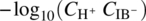 using molar concentrations (in mol/dm3) computed from the liquid‐phase compositions determined by our solid–liquid equilibrium calculations.
Source: Reproduced with permission of American Chemical Society.
19.5.6 Example 5: Polymorphic Transition and Hydrate Formation of Caffeine in Water
Caffeine (CFN) is known to exhibit a polymorphic transition between two different crystalline forms (here denoted as forms I and II). Moreover, a separate solid phase consisting of a hydrate CFN5∙(H2O)4 with a ratio of caffeine to water of 5 : 4 may also form [45, 46]. These factors lead to a complex phase diagram describing the behavior of caffeine in aqueous solutions.
19.5.6.1 System Modeling and Characterization
The molecular structure of caffeine is shown in Figure 19.16. For the purposes of describing the liquid‐phase behavior of this compound in the SAFT‐γ Mie framework, we choose to represent the entire molecule as a single functional group.
FIGURE 19.16 Molecular structure of caffeine (1,3,7‐trimethylpurine‐2,6‐dione). In SAFT‐γ Mie, the entire molecule is modeled as a single functional group.
The necessary SAFT parameters were estimated from published solubility data [47, 48] for caffeine in simple organic solvents. This type of parameter estimation also requires a description of the solid‐phase behavior of caffeine. This was based on the melting point approach described in Section 19.2.4.2 using melting properties reported in the literature [35, 49–51] and summarized in Table 19.4.
TABLE 19.4 Melting Properties of Polymorphic Forms of Caffeine Reported in the Literature [35, 49–51]
| Form I | Form II | ||
| Tm | K | 509.15 | 500.39 |
| Δh[s → l](Tm) | kJ/mol | 21.60 | 22.45 |
| J/mol·K | 101.52 | 101.52 | |
The specific heat capacity difference ![]() is assumed to be constant over the temperature range of interest.
is assumed to be constant over the temperature range of interest.
Figure 19.17 compares the solubilities computed by gSAFT using the estimated SAFT‐γ Mie parameters with the experimental solubility data used for the estimation. As can be seen, a single set of SAFT‐γ Mie parameters leads to a good fit for all four organic solvents, which provides a degree of confidence in employing this molecular model for describing the behavior of caffeine in other systems, such as the aqueous one of interest to this example.
FIGURE 19.17 Comparison of solubilities in organic solvents computed by SAFT‐γ Mie and the experimental data employed for the development of functional group parameters for caffeine [47, 48].
Source: Adapted from Yu et al. [47] and Shalmashi and Golmohammad [48].
The standard SAFT‐γ Mie representation of the water molecule as a single functional group with two electron donor and two electron acceptor association sites was employed. The SAFT‐γ Mie parameters describing the cross‐interactions between the caffeine and water functional groups were estimated from the experimental solubility data for the high temperature polymorph (form I) shown in Figure 19.18a.
FIGURE 19.18 Solid–liquid phase diagram of caffeine with water. Symbols represent experimental data [35, 52] and lines results obtained with gSAFT. (a) Overall phase diagram comprising five distinct regions and six phase boundaries. The Form I solubility data shown as stars were used for fitting the SAFT‐γ Mie unlike interaction parameters between water and caffeine. (b) Low solubility region shown using logarithmic molar fraction scale. The two experimental data points used for the derivation of the empirical free energy function  are shown as filled black circles.
Source: Adapted from Lange et al. [35] and Suzuki et al. [52].
Since caffeine is a non‐ionizable compound, no liquid‐phase reactions need to be considered in this system.
The caffeine hydrate CFN5∙(H2O)4 is assumed to exist only in the solid phase, dissociating into its constituents in the liquid phase:
The solid‐phase free energy of the hydrate was characterized via the procedure described in Section 19.4.3 for compounds that exist only in the solid phase. Two experimental data points (shown as filled black circles in Figure 19.18b) were used to determine the value of the free energy quantity ![]() at two different temperatures, which allows the derivation of the empirical model:
at two different temperatures, which allows the derivation of the empirical model: ![]() (in kJ/mol).
(in kJ/mol).
19.5.6.2 Calculation of Solid–Liquid Phase Diagram
Figure 19.18 shows the solid–liquid phase diagram for caffeine in water computed by gSAFT and compares it with experimental data reported in the literature [35, 52].
Overall, good agreement is observed across the entire phase diagram involving five distinct regions delineated by six phase boundaries. It is worth noting that only a relatively small subset of the experimental data points shown here were used for the characterization of the system (cf. Section 19.5.6.1). All other results shown represent predictions.
Figure 19.18b employs a logarithmic scale for the liquid‐phase molar fraction of caffeine in order to show the low solubility region more clearly. Again, the computed solubilities are in good agreement with the experimental data.
19.5.7 Example 6: Co‐Crystal Solubility of Nicotinamide/Succinic Acid in Mixed Solvents
The system of nicotinamide and succinic acid is an example of the general category of API + coformer systems, where alongside the crystalline forms of the two pure components, a co‐crystal can be formed. In this specific case, the co‐crystal, denoted as NIC2∙SUCC, involves a ratio of nicotinamide to succinic acid of 2 : 1.
The study presented here focuses on the solid–liquid phase diagram of nicotinamide and succinic acid in a 50 : 50 (by weight) mixture of ethanol and water at 298.15 K.
19.5.7.1 System Modeling and Characterization
The molecular structures of nicotinamide and succinic acid are shown in Figure 19.19.
FIGURE 19.19 Molecular structure of (a) nicotinamide (pyridine‐3‐carboxamide) and (b) succinic acid (1,4‐butanedioic acid). In SAFT‐γ Mie, each of these molecules is modeled as a single functional group.
As in the previous example (cf. Section 19.5.6.1), each solute molecule is modeled as a single functional group in the SAFT‐γ Mie framework, and the corresponding parameters are estimated from published experimental solubility data in pure organic solvents and in pure water. The solid‐phase characterization necessary for this estimation was based on the melting point approach described in Section 19.2.4.2 using melting properties reported in the literature [53–55] and summarized in Table 19.5.
TABLE 19.5 Melting Properties of Polymorphic Forms of Nicotinamide and Succinic Reported in the Literature [53–55]
| Nicotinamide | Succinic Acid | ||
| Tm | K | 401.15 | 461.15 |
| Δh[s → l](Tm) | kJ/mol | 28.0 | 38.91 |
| J/mol·K | 78.12 | 69.78 | |
A comparison between the computed and the experimental solubility values is presented in Figure 19.20a for nicotinamide and Figure 19.20b for succinic acid.
FIGURE 19.20 Comparison of solubilities computed by SAFT‐γ Mie and the experimental data employed for the development of functional group parameters for (a) nicotinamide [36, 56] and (b) succinic acid [36, 57, 58].
The solid‐phase free energy of the co‐crystal was characterized via the procedure described in Section 19.4.3 for compounds that exist only in the solid phase. Since our present study is performed entirely at a single temperature of 298.15 K, the free energy quantity ![]() is required only at this temperature and can be determined from a single experimental data point relating to the solubility of the co‐crystal in any solvent that can be described by SAFT‐γ Mie. Here we used the experimentally determined solubility of the co‐crystal in pure ethanol at a temperature of 298.15 K and ambient pressure reported in Ref. [46], obtaining the value
is required only at this temperature and can be determined from a single experimental data point relating to the solubility of the co‐crystal in any solvent that can be described by SAFT‐γ Mie. Here we used the experimentally determined solubility of the co‐crystal in pure ethanol at a temperature of 298.15 K and ambient pressure reported in Ref. [46], obtaining the value ![]() 36.404 kJ/mol.
36.404 kJ/mol.
No liquid‐phase reactions were taken into account in this study.
19.5.7.2 Calculation of Solid–Liquid Phase Diagrams
Figure 19.21 shows solid–liquid phase diagrams of nicotinamide and succinic acid in pure ethanol, pure water, and a 50 : 50 (by weight) mixture of water with ethanol, all computed by gSAFT at a temperature of 298.15 K. Experimental data reported in Ref. [46] are also shown on these diagrams. It is noted that only the single data point shown as a filled black square in Figure 19.21a was used for the characterization of this system (cf. Section 19.5.7.1); all other gSAFT results reported represent predictions.
FIGURE 19.21 Solid–liquid phase diagrams at 298.15 K and 1 atm of nicotinamide. Succinic acid and their (2 : 1) co‐crystal in (a) pure ethanol, (b) pure water, and (c), (d) a 50 : 50 (by weight) mixture of ethanol and water. Symbols represent experimental data [46] and lines results obtained with gSAFT. The single experimental data point used for the estimation of the empirical free energy  is shown as a filled black square in (a).
Source: Lange et al. [46]. http://www.mdpi.com/1420‐3049/21/5/593. Licensed under CC BY 3.0.
Overall, there is good agreement between gSAFT predictions and experimental data. In particular, the results in Figure 19.21c confirm the co‐crystal's significantly increased solubility in the mixed solvent compared to that in pure water or pure ethanol.
19.6 DISCUSSION
The six applications considered in Sections 19.5.2–19.5.7 were selected to illustrate the key aspects of the general framework and methodology for solid–liquid equilibria presented in this chapter. In this section, we revisit each one of these applications and attempt to identify the more general aspects relating to computation of solid–liquid equilibria.
The main compound (fenofibrate) in Example 1 (cf. Section 19.5.2) was fully characterized in terms of already known values of all necessary parameters:
- The SAFT‐γ Mie parameters for its functional groups had already been estimated using fluid‐phase experimental data for unrelated compounds.
- The melting point properties had already been reported in the literature.
In fact, the values of the SAFT‐γ Mie parameters for most solvents of pharmaceutical interest are already present in the gSAFT databank. The example demonstrates that, in such situations, it may be possible to accurately predict solid–liquid equilibria without using any experimental solubility data. Moreover, in general, systems involving mixed solvents pose little additional difficulty either computationally or in terms of the required data since, as the SAFT‐γ Mie EoS is capable of predicting the liquid‐phase chemical potentials, the existence of solvent mixtures affects only the liquid‐phase chemical behavior.
Examples 2 and 3 consider API solubilization in a polymer (PEG). The compounds involved, namely ibuprofen (cf. Section 19.5.3) and ketoprofen (cf. Section 19.5.4), are also fully characterized by already available parameter values. Handling the additional complexity posed by the polymer is straightforward in the context of a group contribution‐based EoS such as SAFT‐γ Mie.
A more interesting challenge encountered in Examples 2 and 3 is the potential presence of API/polymer co‐crystals. The solid‐phase characterization of such co‐crystals does require a small amount of experimental solubility data. In the examples presented here, two data points were sufficient to construct an empirical free energy function as a linear function of temperature, which then allowed the computation of the complete solid–liquid phase diagrams for the API/polymer system. It is worth noting that such a parsimonious reliance on experimental data is made possible by SAFT‐γ Mie's ability to compute accurate values for the ![]() terms on the right‐hand side of Eq. (19.22); this then ensures that the quantity ∆gi computed by Eq. (19.22) is composition independent despite the use of experimentally determined compositions for its evaluation.
terms on the right‐hand side of Eq. (19.22); this then ensures that the quantity ∆gi computed by Eq. (19.22) is composition independent despite the use of experimentally determined compositions for its evaluation.
Example 4 (cf. Section 19.5.5) involved an aqueous system, focusing on API solubility across the entire pH range from strongly acid to strongly alkaline environments. The nonideal behavior of water itself can already be handled well by the ability of SAFT‐γ Mie to describe strongly associating compounds. Also important in this context is SAFT‐γ Mie's handling of ionic species, both on the theoretical level and in terms of the ability to accurately convert formation enthalpies and entropies reported in the literature from one reference state to another. The SAFT‐γ Mie parameterization for the API ion was derived directly from the corresponding parameters of the API itself.
A more significant challenge in such systems is the characterization of the liquid‐phase dissociation of the API. As discussed in Section 19.5.5.2, the common practice of relying on pKa “constants” may be unreliable as the corresponding product of API ion and H+ concentrations is far from constant in at least some parts of the pH spectrum. Instead, the dissociation reaction may be characterized from a small amount of experimental measurements. In this example, the required free energy quantity ![]() at the temperature of interest (298.15 K) was estimated from a single experimental data point, and this was sufficient to characterize the dissociation reaction across the pH spectrum at that temperature. The key to such efficient use of experimental information is SAFT‐γ Mie's ability to compute accurate values for the
at the temperature of interest (298.15 K) was estimated from a single experimental data point, and this was sufficient to characterize the dissociation reaction across the pH spectrum at that temperature. The key to such efficient use of experimental information is SAFT‐γ Mie's ability to compute accurate values for the ![]() terms on the right‐hand side of Eq. (19.24), which makes the value of
terms on the right‐hand side of Eq. (19.24), which makes the value of ![]() independent of the composition at the particular experimental data point being used for its estimation.
independent of the composition at the particular experimental data point being used for its estimation.
Another interesting feature of Example 4 was the potential appearance of a solid API salt hydrate (sodium ibuprofen dihydrate). This was characterized via the use of a single experimental data point to determine the quantity ∆gi via Eq. (19.22). Although the dissociation of API salts gives rise to ionic species in the liquid phase, this does not pose significant challenges beyond those already addressed in the context of co‐crystals.
Examples 5 and 6 (cf. Sections 19.5.6 and 19.5.7, respectively) represent more complex systems combining several of the aspects introduced by earlier examples, such as potential formation of co‐crystals and mixed solvents including strongly associating compounds. The additional element introduced by these examples is the fact that the SAFT‐γ Mie parameters for the solutes are not already known but need to be derived using experimental solubility data. It is important to note that it is possible to use data from solvents that are completely different to those involved in the system under consideration. For instance, the aqueous solubility study reported in Example 5 made use of experimental solubility data in organic solvents. The accuracy of free energy calculations by SAFT‐γ Mie is key to ensuring reliable transferability of information between different systems.
An interesting feature of Example 5 is that, in addition to a hydrate form, there exist two different “neat” polymorphs of the solute. Form II is stable up to the transition temperature of 414.15 K [52], above which Form I becomes stable up to its melting temperature of 509.15 K. In this example, both polymorphs were characterized using melting properties quoted in Ref. [29] that, from the experimental point of view, would imply that the low temperature polymorph, Form II, can be heated up to its melting point without undergoing a solid‐state polymorphic transition to Form I. For systems in which such polymorphic transitions cannot be avoided, the solid‐phase behavior of some polymorphs will need to be characterized using alternative methods, such as those making use of experimental solubility data as described in Section 19.4.2. It is worth noting that these data do not need to relate to the specific solvent(s) for the system under consideration; Eq. (19.17) coupled with SAFT‐γ Mie for the computation of the ![]() term allows an empirical form of the free energy function ∆gi(T) to be determined from available solubility data for that particular polymorph in other solvents.
term allows an empirical form of the free energy function ∆gi(T) to be determined from available solubility data for that particular polymorph in other solvents.
From a computational perspective, the examples demonstrate the ability of gSAFT to determine complex solid–liquid phase diagrams (cf. Figures 19.10, 19.12, 19.18, and 19.21) and also to handle very small concentrations such as those corresponding to ionic species (cf. Figure 19.14d). This is primarily a result of the reliable numerical solution of the phase equilibrium conditions (cf. Section 19.2.2) and the application of the correct stability criteria (cf. Section 19.2.5).
19.7 CONCLUSIONS
This chapter has presented a general framework for solid–liquid equilibrium calculations that covers many of the systems of practical interest to the pharmaceutical industry including those involving diverse types of:
- Solid forms such as simple APIs, API salts, solvates, hydrates, and co‐crystals, as well as multiple polymorphs of these solid forms.
- Solvents, including both water and organic molecules and their mixtures, and polymers.
The framework can describe important aspects such as the effects of pH on solubility, the partial ionization of weakly acidic or basic APIs, and the simultaneous existence of multiple solid and/or liquid phases.
By adopting an approach based on fundamental thermodynamics, all of the above can be handled in a unified manner without the need for diverse concepts such as activity coefficients with respect to multiple reference states, solubility products, acid or base dissociation “constants,” etc. The only thermodynamic properties required are the liquid‐ and solid‐phase chemical potentials of the compounds that potentially exist in the system. In this context, an important development over the last decade has been the emergence of EoS, such as SAFT‐γ Mie, which can describe the fluid‐phase behavior of complex mixtures by taking account of different types of intermolecular interactions. On the other hand, solid‐phase potentials can be evaluated using rigorous thermodynamic expressions involving either the enthalpy and entropy of formation of solid forms or their melting properties.
As demonstrated by the examples presented in Section 19.5, it is now possible to combine the various theoretical elements mentioned above with reliable numerical solvers for phase equilibrium and tests for phase stability, to produce computer codes for the accurate computation of entire solid–liquid phase diagrams for complex systems of pharmaceutical interest.
A key objective of any methodology for the prediction of solid–liquid equilibria is the minimization of the amount of new experimental data that are necessary for characterizing a particular system of interest. Because of its group contribution basis, SAFT‐γ Mie can use information derived from already existing experimental data to be used for the accurate prediction of liquid‐phase behavior, even if the system under consideration involves a completely different set of compounds to those used in the original experiments. On a practical level, the SAFT‐γ Mie parameter databank in gSAFT currently (January 2019) includes parameters for the functional groups describing almost all FDA‐approved solvents [59] for API manufacturing and an increasing number of functional groups occurring in APIs. With the continual addition of more functional groups to this databank, the approach described here becomes applicable to more and more APIs without the need for experimental data for developing descriptions of their liquid‐phase behavior.
Unfortunately, at present there is no general theoretical approach that will allow similarly accurate cross‐compound transferability of information for solid phases. However, as explained in Section 19.4, by combining small amounts of experimental solubility data for the solid forms of interest with SAFT‐γ Mie liquid‐phase predictions, it is possible to predict solid–liquid equilibria for these forms over wide ranges of conditions and/or in conjunction with different solvents. The practical examples presented in Section 19.5 provide some evidence for the applicability and effectiveness of this approach.
19.A USING FORMATION PROPERTIES IN THE INFINITE DILUTION STATE
Ionic compounds in aqueous systems cannot exist in pure form. Accordingly, from the perspective of relating thermodynamic theory to experimentally observable quantities, it is preferable to consider their properties with respect to an “infinite dilution” reference state corresponding to the limit of their presence tending to zero (or, equivalently, the molar fraction of water, xw, tending to 1) in an aqueous solution at standard T⊖, P⊖.
The chemical potential of ionic compound i generally depends on the logarithm of the corresponding molar fraction xi (cf. the term +RT ln(xi) in Eq. 19.9). This dependence needs to be removed in order to ensure that the partial molar Gibbs free energy ![]() at the reference state has a finite value. Historically, three different approaches have been proposed to achieve this, each making use of a different measure of ionic concentration:
at the reference state has a finite value. Historically, three different approaches have been proposed to achieve this, each making use of a different measure of ionic concentration:
- Molar fraction‐based reference state:
- Molality‐based reference state:(19.A.1b)
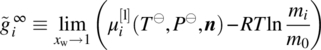
where mi ≡ xi/xwMw denotes the molality, with Mw being the molecular weight of water and m0 = 1 mol/kg.
- Molarity‐based reference state:
where Ci ≡ xiρw/Mw denotes the molarity (molar concentration), with ρw being the mass density (in kg/dm3) of pure water at T⊖, P⊖ and C0= 1 mol/dm3.
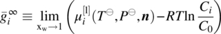
The free energy ![]() and enthalpy
and enthalpy ![]() of formation in the infinite dilution reference state that are typically reported in the literature are related to
of formation in the infinite dilution reference state that are typically reported in the literature are related to ![]() via the standard thermodynamic relations:
via the standard thermodynamic relations:
It can be shown that, while each of the three infinite dilution reference states leads to a different value for ![]() , they all result in the same value for
, they all result in the same value for ![]() .
.
Using Eqs. (19.8) and (19.9) for the chemical potential ![]() appearing in Eqs. (19.A.1a)–(19.A.1c), we can derive the following relations between the ideal gas formation entropy and the formation entropies in the various infinite dilution reference states:
appearing in Eqs. (19.A.1a)–(19.A.1c), we can derive the following relations between the ideal gas formation entropy and the formation entropies in the various infinite dilution reference states:
- Molar fraction‐based reference state:
- Molality‐based reference state:
- Molarity‐based reference state:
where
 is the residual chemical potential of compound i in an infinitely diluted composition. In practical terms, this can be computed by applying an EoS such as SAFT‐γ Mie to a binary mixture comprising water and compound i and setting the corresponding molar fractions to xw = 1 and xi = 0, respectively.
In all three cases, the ideal gas enthalpy of formation ![]() can be obtained from the corresponding infinite dilution values
can be obtained from the corresponding infinite dilution values ![]() via the equation
via the equation
In summary, Eqs. (19.A.3a)–(19.A.3c) and (19.A.4), coupled with an EoS to compute the residual term ![]() , allow the determination of the ideal gas formation properties
, allow the determination of the ideal gas formation properties ![]() and
and ![]() from experimentally derived values
from experimentally derived values ![]() and
and ![]() in any one of the commonly used infinite dilution reference states.
in any one of the commonly used infinite dilution reference states.
19.B SAFT‐γ MIE FUNCTIONAL GROUP DECOMPOSITION
The functional group decomposition of the compounds involved in the examples of Section 19.5 within the SAFT‐γ Mie framework is shown in the table below.
| Species | Functional Group Decomposition | ||||||||||||||||
| 1‐Butanol | 1 | CH3 | 3 | CH2 | 1 | OH | |||||||||||
| 1‐Propanol | 1 | CH3 | 2 | CH2 | 1 | OH | |||||||||||
| 2‐Propanol | 2 | CH3 | 1 | CH | 1 | OH_Sec | |||||||||||
| Ethanol | 1 | CH3 | 1 | CH2 | 1 | OH | |||||||||||
| Ethyl acetate | 2 | CH3 | 1 | CH2 | 1 | COO | |||||||||||
| Toluene | 1 | aCCH3 | 5 | aCH | |||||||||||||
| Acetone | 1 | CH3COCH3 | |||||||||||||||
| Acetonitrile | 1 | CH3CN | |||||||||||||||
| Cyclohexane | 6 | cyCH2 | |||||||||||||||
| Methanol | 1 | CH3OH | |||||||||||||||
| Water | 1 | H2O | |||||||||||||||
| Caffeine | 1 | C8H10N4O2 | |||||||||||||||
| Fenofibrate | 1 | aCCOaC | 8 | aCH | 1 | aCCl | 1 | aCO | 1 | COOH | 1 | COO | 4 | CH3 | 1 | CH | |
| Ibuprofen | 3 | CH3 | 1 | CH | 1 | aCCH2 | 1 | aCCH | 4 | aCH | 1 | COOH | |||||
| Ibuprofen ion | 3 | CH3 | 1 | CH | 1 | aCCH2 | 1 | aCCH | 4 | aCH | 1 | COO─ | |||||
| Ketoprofen | 1 | aCCOaC | 1 | CH3 | 1 | aCCH | 9 | aCH | 1 | COOH | |||||||
| Nicotinamide | 1 | C6H6N2O | |||||||||||||||
| PEG 10000 | 454 | CH2 | 226 | cO | 2 | OH | |||||||||||
| PEG 6000 | 272 | CH2 | 135 | cO | 2 | OH | |||||||||||
| Succinic acid | 1 | C4H6O4 | |||||||||||||||
| H+ | 1 | H+ | |||||||||||||||
| OH− | 1 | OH− | |||||||||||||||
| Na+ | 1 | Na+ | |||||||||||||||
| Cl− | 1 | Cl− | |||||||||||||||
REFERENCES
- 1. Sugano, K. (2012). Biopharmaceutics Modeling and Simulations: Theory, Practice, Methods and Applications. Hoboken: Wiley.
- 2. Shan, N. and Zaworotko, M.J. (2008). The role of cocrystals in pharmaceutical science. 2. 3. Drug Discov. Today 13: 440–446.
- 3. Qiao, N., Li, M., Schlindwein, W. et al. (2011). Pharmaceutical cocrystals: an overview. Int. J. Pharm. 419: 1–11.
- 4. Lu, J. and Rohani, S. (2009). Polymorphism and crystallization of active pharmaceutical ingredients (APIs). Curr. Med. Chem. 16: 884–905.
- 5. Kiesow, K., Tumaka, F., and Sadowski, G. (2008). Experimental investigation and prediction of oiling out during crystallization process. J. Cryst. Growth 310: 4163–4168.
- 6. Lu, J., Li, Y.‐P., Wang, J. et al. (2012). Crystallization of an active pharmaceutical ingredient that oils out. Sep. Purif. Technol. 96: 1–6.
- 7. Michelsen, M.L. and Mollerup, J.M. (2007). Thermodynamic Models: Fundamentals & Computational Aspects. Holte, Denmark: Tie‐Line Publications.
- 8. Chen, C.‐C. (2011). Molecular thermodynamics for pharmaceutical process modeling and simulation. In: Chemical Engineering in the Pharmaceutical Industry (ed. D.J. am Ende), 505–514. Hoboken: Wiley.
- 9. Paricaud, P., Galindo, A., and Jackson, G. (2004). Modeling the cloud curves and the solubility of gases in amorphous and semicrystalline polyethylene with the SAFT‐VR approach and Flory theory of crystallization. Ind. Eng. Chem. Res. 43: 6871–6889.
- 10. Michelsen, M.L. (1982). The isothermal flash problem. Part I. Stability. Fluid Phase Equilib. 9: 1–19.
- 11. Pereira, F.E., Jackson, G., Galindo, A., and Adjiman, C.S. (2010). A duality‐based optimisation approach for the reliable solution of (P, T) phase equilibrium in volume‐composition space. Fluid Phase Equilib. 299 (1): 1–23.
- 12. Pereira, F.E., Jackson, G., Galindo, A., and Adjiman, C.S. (2012). The HELD algorithm for multicomponent, multiphase equilibrium calculations with generic equations of state. Comput. Chem. Eng. 36: 99–118.
- 13. McDonald, C.M. and Floudas, C.A. (1995). Global optimization for the phase stability problem. AIChE J. 41 (7): 1798–1814.
- 14. Jackson, G., Chapman, W.G., and Gubbins, K.E. (1988). Phase equilibria of associating fluids – spherical molecules with multiple bonding sites. Mol. Phys. 65 (1): 1–31.
- 15. Chapman, W.G., Gubbins, K.E., Jackson, G., and Radosz, M. (1990). New reference equation of state for associating liquids. Ind. Eng. Chem. Res. 29 (8): 1079–1721.
- 16. Economou, I. (2002). Statistical associating fluid theory: a successful model for the calculation of thermodynamic and phase equilibrium properties of complex fluid mixtures. Ind. Eng. Chem. Res. 41: 953–962.
- 17. Müller, E.A. and Gubbins, K.E. (2001). Molecular‐based equations of state for associating fluids: a review of SAFT and related approaches. Ind. Eng. Chem. Res. 40: 22193–22211.
- 18. McCabe, C. and Galindo, A. (2011). SAFT associating fluids and fluid mixtures. In: Applied Thermodynamics of Fluids (ed. A.R.H. Goodwin, J.V. Sengers and C.J. Peters), 215–279. London: Royal Society of Chemistry.
- 19. Papaioannou, V., Lafitte, T., Avendaño, C. et al. (2014). Group contribution methodology based on the statistical associating fluid theory for heteronuclear molecules formed from Mie segments. J. Chem. Phys. 140: 054107.
- 20. Dufal, S., Lafitte, T., Haslam, A.J. et al. (2015). The A in SAFT: developing the contribution of association to the Helmholtz free energy within a Wertheim TPT1 treatment of generic Mie fluids. Mol. Phys. 113: 948–984.
- 21. Sadeqzadeh, M., Papaioannou, V., Dufal, S. et al. (2016). The development of unlike induced association‐site models to study the phase behaviour of aqueous mixtures comprising acetone, alkanes and alkyl carboxylic acids with the SAFT‐γ Mie group contribution methodology. Fluid Phase Equilib. 407: 39–57.
- 22. Joback, K.G. and Reid, R.C. (1987). Estimation of pure‐component properties from group contributions. Chem. Eng. Commun. 57: 233–243.
- 23. Gracin, S. and Rasmuson, Å.C. (2002). Solubility of phenylacetic acid, p‐hydroxyphenylacetic acid, p‐aminophenylacetic acid, p‐hydroxybenzoic acid, and ibuprofen in pure solvents. J. Chem. Eng. Data 47 (6): 1379–1383.
- 24. Wang, S., Song, Z., Wang, J. et al. (2010). Solubilities of ibuprofen in different pure solvents. J. Chem. Eng. Data 55 (11): 5283–5285.
- 25. Domanska, U., Pobudkowska, A., Pelczarska, A., and Gierycz, P. (2009). pKa and solubility of drugs in water, ethanol, and 1‐octanol. J. Phys. Chem. B 113 (26): 8941–8947.
- 26. Garzon, L.C. and Martınez, F. (2004). Temperature dependence of solubility for ibuprofen in some organic and aqueous solvents. J. Solut. Chem. 33 (11): 1379–1395.
- 27. Process Systems Enterprise Ltd. (2018). gPROMS advanced thermodynamics [Online]. https://www.psenterprise.com/products/gsaft (accessed 5 January 2018).
- 28. Process Systems Enterprise Ltd. (2018). gPROMS platform [Online]. https://www.psenterprise.com/products/gproms (accessed 5 January 2018).
- 29. Gill‐Villegas, A., Galindo, A., Whitehead, P.J. et al. (1997). Statistical associating fluid theory for chain molecules with attractive potentials of variable range. J. Chem. Phys. 106: 4168.
- 30. Galindo, A., Davies, L.A., Gil‐Villegas, A., and Jackson, G. (1998). The thermodynamics of mixtures and the corresponding mixing rules in the SAFT‐VR approach for potentials of variable range. Mol. Phys. 93 (2): 241–252.
- 31. Gross, J. and Sadowski, G. (2001). Perturbed‐chain SAFT: an equation of state based on a perturbation theory for chain molecules. Ind. Eng. Chem. Res. 40: 1244–1260.
- 32. Gross, J. and Sadowski, G. (2002). Application of the perturbed‐chain SAFT equation of state to associating systems. Ind. Eng. Chem. Res. 41: 5510–5515.
- 33. Cuevas, J., Llovell, F., Galindo, A. et al. (2011). Solid–liquid equilibrium using the SAFT‐VR equation of state: solubility of naphthalene and acetic acid in binary mixtures and calculation of phase diagrams. Fluid Phase Equilib. 306: 137–147.
- 34. Prudic, A., Ji, Y., and Sadowski, G. (2014). Thermodynamic phase behavior of API/polymer solid dispersions. Mol. Pharm. 11: 2294–2304.
- 35. Lange, L., Schleinitz, M., and Sadowski, G. (2016). Predicting the effect of pH on stability and solubility of polymorphs, hydrates, and cocrystals. Cryst. Growth Des. 16 (7): 4136–4147.
- 36. Lange, L., Lehmkemper, K., and Sadowski, G. (2016). Predicting the aqueous solubility of pharmaceutical cocrystals as function of pH and temperature. Cryst. Growth Des. 16 (5): 2726–2740.
- 37. Watterson, S., Hudson, S., Svärd, M., and Rasmuson, Å.C. (2014). Thermodynamics of fenofibrate and solubility in pure organic solvents. Fluid Phase Equilib. 367: 143–150.
- 38. Sun, H., Liu, B., Liu, P. et al. (2016). Solubility of fenofibrate in different binary solvents: experimental data and results of thermodynamic modeling. J. Chem. Eng. Data 61 (9): 3177–3183.
- 39. Khan, G.M. and Jiabi, Z. (1998). Preparation, characterization, and dissolution studies of ibuprofen solid dispersions using polyethylene glycol (PEG), talc, and PEG‐talc as dispersion carriers. Drug Dev. Ind. Pharm. 24 (5): 455–462.
- 40. Wassvik, C.M., Holmén, A.G., Bergström, C.A. et al. (2006). Contribution of solid‐state properties to the aqueous solubility of drugs. Eur. J. Pharm. Sci. 29 (3–4): 294–305.
- 41. Margarit, M.V., Rodriguez, I.C., and Cerezo, A. (1994). Physical characteristics and dissolution kinetics of solid dispersions of ketoprofen and polyethylene glycol 6000. Int. J. Pharm. 108: 101–107.
- 42. Avdeef, A., Berger, C.M., and Brownell, C. (2000). pH‐metric solubility. 2: correlation between the acid‐base titration and the saturation shake‐flask solubility‐pH methods. Pharm. Res. 17 (1): 85–89.
- 43. Shaw, L.R., Irwin, W.J., Grattan, T.J., and Conway, B.R. (2005). The effect of selected water‐soluble excipients on the dissolution of paracetamol and ibuprofen. Drug Dev. Ind. Pharm. 31: 515–525.
- 44. Censi, R., Martena, V., Hoti, E. et al. (2013). Sodium ibuprofen dihydrate and anhydrous: study of the dehydration and hydration mechanisms. J. Therm. Anal. Calorim. 111: 2009–2018.
- 45. Wagman, D.D., Evans, W.H., Parker, V.B. et al. (1982). The NBS tables of chemical thermodynamic properties. Selected values for inorganic and C1 and C2 organic substances in SI units. National Standard Reference Data System.
- 46. Lange, L., Heisel, S., and Sadowski, G. (2016). Predicting the solubility of pharmaceutical cocrystals in solvent/anti‐solvent mixtures. Molecules 21: 593.
- 47. Yu, Z.Q., Chow, P.S., and Tan, R.B.H. (2010). Operating regions in cooling cocrystallization of caffeine and glutaric acid in acetonitrile. Cryst. Growth Des. 10 (5): 2382–2387.
- 48. Shalmashi, A. and Golmohammad, F. (2010). Solubility of caffeine in water, ethyl acetate, ethanol, carbon tetrachloride, dichloromethane, and acetone between 298 and 323 K. Lat. Am. Appl. Res. 40: 283–285.
- 49. Cesaro, A. and Starec, G. (1980). Thermodynamic properties of caffeine crystal forms. J. Chem. Phys. 84: 1345–1346.
- 50. Bothe, H. and Cammenga, H.K. (1979). Phase transitions and thermodynamic properties of anhydrous caffeine. J. Thermal Anal. 16: 267–275.
- 51. Kolska, Z., Kukal, J., Zabransky, M., and Ruzicka, V. (2008). Estimation of the heat capacity of organic liquids as a function of temperature by a three‐level group contribution method. Ind. Eng. Chem. Res. 47: 2075–2085.
- 52. Suzuki, E., Shirotani, K.‐I., Tsuda, Y., and Sekiguchi, K. (1985). Water content and dehydration behavior of crystalline caffeine hydrate. Chem. Pharm. Bull. 33 (11): 5028–5035.
- 53. Laube, F.S., Klein, T., and Sadowski, G. (2015). Partition coefficients of pharmaceuticals as functions of temperature and pH. Ind. Eng. Chem. Res. 54: 3968–3975.
- 54. Riipinen, I., Svenningsson, B., Bilde, M. et al. (2006). A method for determining thermophysical properties of organic material in aqueous solutions: succinic acid. Atmos. Res. 82: 579–590.
- 55. Marrero, J. and Abildskov, J. (2003). Solubility and Related Properties of Large Complex Chemicals, vol. 15. DECHEMA.
- 56. Wu, H., Dang, L., and Wei, H. (2014). Solid‐liquid phase equilibrium of nicotinamide in different pure solvents: measurements and thermodynamic modeling. Ind. Eng. Chem. Res. 53 (4): 1707–1711.
- 57. Zhang, H., Yin, Q., Liu, Z. et al. (2014). An odd‐even effect on solubility of dicarboxylic acids in organic solvents. J. Chem. Thermodyn. 77: 91–97.
- 58. Yu, Q., Black, S., and Wei, H. (2009). Solubility of butanedioic acid in different solvents at temperatures between 283 K and 333 K. J. Chem. Eng. Data 54 (7): 2123–2125.
- 59. International Council for Harmonisation of Technical Requirements for Pharmaceuticals for Human Use (2016). Impurities: Guideline for Residual Solvents – Q3C(R6).